ORCCA Exponential and Logarithmic Functions Chapter Review

Section 14.4 Exponential and Logarithmic Functions Chapter Review

Subsection 14.4.1 Exponential Functions

Graph Exponential Functions.

In Section 14.1, we learned that an exponential function is a function of the form

\begin{equation*} f\left(x\right)={b}^{x}\text{,} \end{equation*}

where $b>0$ and $b\ne 1\text{.}$

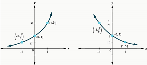
We also learned that the graph of an exponential function has the following properties:

Table 14.4.1. Properties of the Graph of $f(x)=b^x$

when $b>1$		when $0<b<1$
Domain	$\left(-\infty ,\infty \right)$	Domain	$\left(-\infty ,\infty \right)$
Range	$\left(0,\infty \right)$	Range	$\left(0,\infty \right)$
$x$-intercept	none	$x$-intercept	none
$y$-intercept	$\left(0,1\right)$	$y$-intercept	$\left(0,1\right)$
Contains	$\left(1,b\right), \left(-1,\frac{1}{b}\right)$	Contains	$\left(1,b\right), \left(-1,\frac{1}{b}\right)$
Asymptote	$x$-axis, the line $y=0$	Asymptote	$x$-axis, the line $y=0$
Basic shape	increasing	Basic shape	decreasing

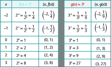
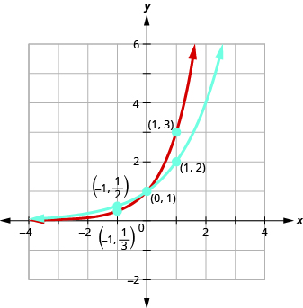
Graphs of the functions y=b^x when b>0 and y=b^x when b is between 0 and 1, graphed side by side. — Figure 14.4.2.

Example 14.4.3.

On the same coordinate system graph $f\left(x\right)={2}^{x}$ and $g\left(x\right)={3}^{x}\text{.}$

Explanation

We will use point plotting to graph the functions.

A table of values for graphing f(x)=2^x and g(x)=3^x. — Figure 14.4.4.

A graph of f(x)=2^x, in blue, and g(x)=3^x, in red, graphed on the same coordinate system. — Figure 14.4.5.

Example 14.4.6.

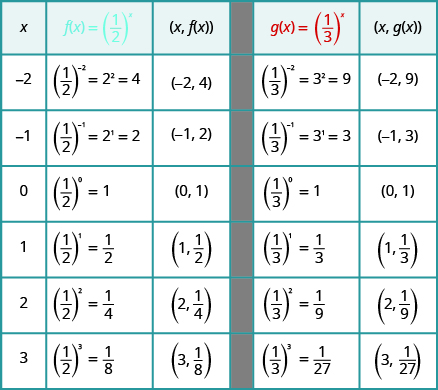
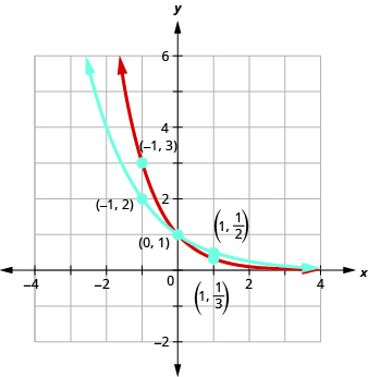
On the same coordinate system, graph $f\left(x\right)={\left(\frac{1}{2}\right)}^{x}$ and $g\left(x\right)={\left(\frac{1}{3}\right)}^{x}\text{.}$

Explanation

We will use point plotting to graph the functions.

A table of values for f(x)=(1/2)^x and g(x)=(1/3)^x. — Figure 14.4.7.

A graph of f(x)=(1/2)^x, in blue, and g(x)=(1/3)^x, in red, graphed on the same coordinate system. — Figure 14.4.8.

Natural Base e.

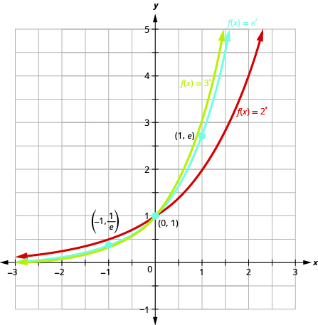
In this section, we learned about the natural number $e\text{,}$ which is an irrational number like $\pi$ whose value is $e\approx 2.718281827..\text{..}$ The graph of the function $f(x)=e^x\text{,}$ compared to functions $g(x)=2^x$ and $h(x)=3^x$ is given in the figure below:

Graph of the function f(x)=e^x, in blue, on the same coordinate system as g(x)=2^x, in red, and h(x)=3^x, in green. — Figure 14.4.9.

Use Exponential Models in Applications.

In this section, we also learned how exponential functions can be used in the real world to model things like compound interest and exponential growth.

Compound Interest.

There are two formulas that are used to determine the balance in the account when interest is earned. If a principal, $P\text{,}$ is invested at an interest rate, $r$ (in decimal form), for $t$ years, the new balance, $A\text{,}$ will depend on how often the interest is compounded. If the interest is compounded $n$ times a year we use the formula $A=P\left(1+\frac{r}{n}\right)^{nt}\text{.}$ If the interest is compounded continuously, we use the formula $A=P{e}^{rt}\text{.}$ These are the formulas for compound interest.

For a principal, $P\text{,}$ invested at an interest rate, $r$ (in decimal form), for $t$ years, the new balance, $A\text{,}$ is:

\begin{align*} A=P\left(1+\frac{r}{n}\right)^{nt}\amp \text{when compounded } n \text{ times a year.} \end{align*}

\begin{align*} A=P{e}^{rt}\amp \text{when compounded continuously.} \end{align*}

Example 14.4.10.

A total of $\$10{,}000$ was invested in a college fund for a new grandchild. If the interest rate is $5\%\text{,}$ how much will be in the account in $18$ years by each method of compounding?

compound quarterly
compound monthly
compound continuously

Explanation

Table 14.4.11.

	$A=\text{ ?}$
Identify the values of each variable in the formulas.	$P=\$10{,}000$
Be sure to express the percent as a decimal.	$r=0.05$
	$t=18$ years
a.
For quarterly compounding, $n=4$	$A=P\left(1+\frac{r}{n}\right)^{nt}$
There are $4$ quarters per year.
Substitute the values in the formula.	$A=10{,}000\left(1+\frac{0.05}{4}\right)^{4\cdot 18}$
Compute the amount, being careful to follow
the order of operation as you enter the
expression into your calculator.
Round to the nearest cent.	$A=\$24{,}459.20$

b.
For monthly compounding, $n=12$	$A=P\left(1+\frac{r}{n}\right)^{nt}$
There are $12$ months per year.
Substitute the values in the formula.	$A=10{,}000\left(1+\frac{0.05}{12}\right)^{12\cdot 18}$
Compute and round to the nearest cent.	$A=\$24{,}550.08$

c.
For compounding continuously,	$A=Pe^{nt}$
Substitute the values in the formula.	$A=e^{0.05\cdot 18}$
Compute and round to the nearest cent.	$A=\$24{,}596.03$

Exponential Growth and Decay.

Other topics that are modeled by exponential functions involve growth and decay. Both also use the formula $A=P{e}^{rt}$ we used for the growth of money. For growth and decay, generally we use ${A}_{0}\text{,}$ as the original amount instead of calling it $P\text{,}$ the principal. We see that exponential growth has a positive rate of growth and exponential decay has a negative rate of growth.

For an original amount, ${A}_{0}\text{,}$ that grows or decays at a rate, $r\text{,}$ for a certain time, $t\text{,}$ the final amount, $A\text{,}$ is:

\begin{equation*} A={A}_{0}{e}^{rt} \end{equation*}

Example 14.4.12.

Chris is a researcher at the Center for Disease Control and Prevention and he is trying to understand the behavior of a new and dangerous virus. He starts his experiment with $100$ of the virus that grows at a rate of $25\%$ per hour. He will check on the virus in $24$ hours. How many viruses will he find?

Explanation

Table 14.4.13.

Identify the values of each variable in the formulas.	$A=\text{ ?}$
Be sure to put the percent in decimal form.	$A_{0}=100$
Be sure the units match - the rate is per hour,	$r=0.25\text{/hour}$
the time is in hours.	$t=24\text{ hours}$

Substitute the values in the formula: $A=A_{0}e^{rt}$	$A=100e^{0.25\cdot 24}$
Compute the amount.	$A=40,342.88$
Round to the nearest whole virus.	$A=40,343$
answer the question.	The researcher will find 40,343 viruses.

Subsection 14.4.2 Logarithmic Functions

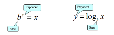
In Section 14.2, we learned how logarithmic functions are related to exponential functions and, in particular, how to use that relationship to convert logarithmic equations into exponential equations or convert exponential equations into logarithmic equations.

The following illustration can be useful in identifying the base and exponent in either form, which is key to making those conversions:

Diagram of exponential equation versus logarithmic equation, pointing out the base and exponent in each. — Figure 14.4.14.

Example 14.4.15. Converting from Logarithmic Form to Exponential Form.

Write the following logarithmic equations in exponential form.

$\displaystyle \mathrm{log}_{5}\left(\sqrt[3]{5}\right)=\frac{1}{3}$
$\displaystyle \mathrm{log}_{4}\left(64\right)=3$

Explanation

First, identify the values of $b\text{,}$ $y\text{,}$ and, $x\text{.}$ Then, write the equation in the form $b^y=x\text{.}$

$\mathrm{log}_{5}\left(\sqrt[3]{5}\right)=\frac{1}{3}$

Here, $b=5\text{,}$ $y=\frac{1}{3}\text{,}$ and $x=\sqrt[3]{5}\text{.}$ Therefore, the equivalent exponential equation is $5^{\frac{1}{3}}=\sqrt[3]{5}\text{.}$
$\mathrm{log}_{4}\left(64\right)=3$

Here, $b=4\text{,}$ $y=3\text{,}$ and $x=64\text{.}$ Therefore, the equation $\mathrm{log}_{4}\left(64\right)=3$ is equivalent to $4^3=64\text{.}$

Example 14.4.16. Converting from Exponential Form to Logarithmic Form.

Write the following exponential equations in logarithmic form.

$\displaystyle 6^2=36$
$\displaystyle 5^{-3}=\frac{1}{125}$

Explanation

First, identify the values of $b\text{,}$ $y\text{,}$ and $x\text{.}$ Then, write the equation in the form $y=\mathrm{log}_{b}\left(x\right)\text{.}$

$6^2=36$

Here, $b=6\text{,}$ $y=2\text{,}$ and $x=36\text{.}$ Therefore, the equation $6^2=36$ is equivalent to $\mathrm{log}_{6}\left(36\right)=2\text{.}$
$5^{-3}=\frac{1}{125}$

Here, $b=5\text{,}$ $y=-3\text{,}$ and $x=\frac{1}{125}\text{.}$ Therefore, the equation $5^{-3}=\frac{1}{125}$ is equivalent to $\mathrm{log}_{5}\left(\frac{1}{125}\right)=-3\text{.}$

We also learned about special logarithms called common and natural logarithms:

For $x>0\text{,}$

\begin{equation*} y=\mathrm{log}\left(x\right)\text{ is equivalent to }10^y=x \end{equation*}

We read $\mathrm{log}\left(x\right)$ as, “the logarithm with base $10$ of $x$” or “log base $10$ of $x\text{.}$” This is called the common logarithm.

For $x>0\text{,}$

\begin{equation*} y=\mathrm{ln}\left(x\right)\text{ is equivalent to }{e}^{y}=x \end{equation*}

We read $\mathrm{ln}\left(x\right)$ as, “the logarithm with base $e$ of $x$” or “the natural logarithm of $x\text{.}$” This is called the natural logarithm.

Example 14.4.17. Finding the Value of a Common Logarithm Mentally.

Solve $y=\mathrm{log}\left(10{,}000\right)$ without using a calculator.

Explanation

First we rewrite the logarithm in exponential form: $10^y=10{,}000\text{.}$ Next, we ask, “To what exponent must $10$ be raised in order to get $10{,}000\text{?}$” We know $10^4=10{,}000\text{.}$ Therefore, $y=\mathrm{log}\left(10{,}000\right)=4\text{.}$

Example 14.4.18. Converting from Natural Logarithmic Form to Exponential Form.

Write the equation $\mathrm{ln}\left(P\right)=5$ in exponential form.

Explanation

First, identify the values of $b\text{,}$ $y\text{,}$ and $x\text{.}$ Then, write the equation in the form $b^y=x\text{.}$

$\mathrm{ln}\left(P\right)=5$

Here, $b=e\text{,}$ $y=5$ and $x=P\text{.}$ Therefore, the equation $\mathrm{ln}\left(P\right)=5$ is equivalent to $e^5=P\text{.}$

Subsection 14.4.3 Using the Change-of-Base Formula

In Section 14.3, we learned a formula that would allow us to rewrite logarithmic expressions, which are not of base $10$ or base $e\text{,}$ so that we are able to evaluate the expression using a scientific calculator.

The Change-of-Base Formula introduces a new base $a\text{.}$ This can be any base $a$ we want where $a\gt 0, a\neq 1\text{.}$ Because our calculators have keys for logarithms base $10$ and base $e\text{,}$ we will typically choose to write the Change-of-Base Formula with the new base as either $10$ or $e\text{.}$

Definition 14.4.19. Change-of-Base Formula.

For any logarithmic bases $a\text{,}$ $b\text{,}$ $M\gt 0$ and $\neq 1\text{,}$

\begin{gather*} \mathrm{log}_{b}M=\frac{\mathrm{log}_{a}M}{\mathrm{log}_{a}b}\\ \\ \text{new base } a \end{gather*}

\begin{gather*} \mathrm{log}_{b}M=\frac{\mathrm{log}M}{\mathrm{log}b}\\ \\ \text{new base } 10 \end{gather*}

\begin{gather*} \mathrm{log}_{b}M=\frac{\mathrm{ln}M}{\mathrm{ln}b}\\ \\ \text{new base } e \end{gather*}

Example 14.4.20.

Rounding to three decimal places, approximate $\mathrm{log}_{5}172\text{.}$

Explanation

We want to evaluate $\mathrm{log}_{5}172\text{,}$ which is not base $10$ or base $e\text{.}$ So we can't enter it directly into our calculator at this point, but we can use the Change-of-Base Formula to rewrite it into either base $10$ or base $e\text{.}$ Then, we will be able to enter it into the calculator.

According to the Change-of-Base Formula,

\begin{equation*} \mathrm{log}_{b}M=\frac{\mathrm{log}M}{\mathrm{log}b}\text{ or }\mathrm{log}_{b}M=\frac{\mathrm{ln}M}{\mathrm{ln}b} \end{equation*}

To use this formula, we need to identify that $b=5$ and $M=172\text{.}$

Now let's choose log base $10$ to rewrite the log.

\begin{equation*} \mathrm{log}_{5}172=\frac{\mathrm{log}172}{\mathrm{log}5}\text{.} \end{equation*}

Enter the expression $\frac{\mathrm{log}172}{\mathrm{log}5}$ in the calculator using the log button for base $10\text{.}$

Then, rounding to three decimal places, we have

\begin{equation*} \mathrm{log}_{5}172\approx 3.198\text{.} \end{equation*}

Exercises 14.4.4 Exercises

Evaluate Exponential Functions

1.

For the function $f(x)= 7^x,$ calculate the following function values:

$f(-3)=$

$f(-1)=$

$f(0)=$

$f(1)=$

$f(3)=$

2.

For the function $f(x)= 3^x,$ calculate the following function values:

$f(-3)=$

$f(-1)=$

$f(0)=$

$f(1)=$

$f(3)=$

Graph Exponential Functions

In the following exercises, graph each exponential function.

3.

$f(x)=6^x$

4.

$f(x)=(\frac{1}{2})^x$

5.

Graph the functions on the same coordinate system: $f\left(x\right)={4}^{x} and g\left(x\right)={4}^{x-1}\text{.}$

Compound Interest

6.

The compound interest formula is

$\displaystyle{ A(t) = P(1+\frac{r}{n})^{nt} }$

where $A(t)$ models the amount of money, $t$ is the number of years, $P$ is the initial amount, $r$ is the annual interest and $n$ is the number of compoundings per year.

Jenny saved ${\$47{,}000.00}$ in an account with an annual interest of $3.8\%\text{.}$ Answer the following questions:

1) The amount of money in the account would be after $11$ years, if the interest is compounded yearly.

2) The amount of money in the account would be after $11$ years, if the interest is compounded quarterly.

3) The amount of money in the account would be after $11$ years, if the interest is compounded monthly.

4) The amount of money in the account would be after $11$ years, if the interest is compounded daily (assuming that year has 365 days).

7.

The compound interest formula is

$\displaystyle{ A(t) = P(1+\frac{r}{n})^{nt} }$

where $A(t)$ models the amount of money, $t$ is the number of years, $P$ is the initial amount, $r$ is the annual interest and $n$ is the number of compoundings per year.

Maria saved ${\$16{,}000.00}$ in an account with an annual interest of $2\%\text{.}$ Answer the following questions:

1) The amount of money in the account would be after $7$ years, if the interest is compounded yearly.

2) The amount of money in the account would be after $7$ years, if the interest is compounded quarterly.

3) The amount of money in the account would be after $7$ years, if the interest is compounded monthly.

4) The amount of money in the account would be after $7$ years, if the interest is compounded daily (assuming that year has 365 days).

Population Growth

8.

In the last ten years, the population of Axtonia has grown at a rate of $2.3\%$ per year to $57{,}768\text{.}$ If this rate continues, what will be the population in $10$ more years?

The population will be .

9.

In the last twenty years, the population of Charizzo has grown at a rate of $0.4\%$ per year to $673{,}426\text{.}$ If this rate continues, what will be the population in $20$ more years?

The population will be .

Logarithmic Functions

For the following exercises, rewrite each equation in exponential form.

10.

${\mathrm{log}}_{N}\left(75\right)=3$

11.

${\mathrm{log}}_{9}\left(P\right)=Q$

12.

$\mathrm{ln}\left(a\right)=b$

13.

$\mathrm{log}\left(200\right)=H$

For the following exercises, rewrite each equation in logarithmic form.

14.

${10}^{R}=M$

15.

${6}^{b}=c$

16.

${X}^{Y}=Z$

17.

${e}^{\frac{1}{2}}=\sqrt{e}$

For the following exercises, evaluate the logarithmic expression without using a calculator.

18.

${\mathrm{log}}_{27}\left(\sqrt[5]{27}\right)=$

19.

${\mathrm{log}}_{3}\left(\frac{1}{9}\right)=$

20.

${\mathrm{log}}_{8}\left(2\right)=$

21.

${\mathrm{log}}_{4}\left(\frac{1}{64}\right)=$

For the following exercises, evaluate each expression using a calculator. Round to the nearest thousandth.

22.

$\mathrm{ln}\left(15{,}425\right) \approx$

23.

$\mathrm{log}\left(0.564\right) \approx$

Using Change-of-Base Formula

In the following exercises, use the Change-of-Base Formula to approximate each logarithm, rounding to three decimal places.

24.

$\mathrm{log}_{4}914 \approx$

25.

$\mathrm{log}_{6}470 \approx$

26.

$\mathrm{log}_{5}0.25 \approx$

27.

$\mathrm{log}_{15}0.24 \approx$

when \(b>1\)		when \(0<b<1\)
Domain	\(\left(-\infty ,\infty \right)\)	Domain	\(\left(-\infty ,\infty \right)\)
Range	\(\left(0,\infty \right)\)	Range	\(\left(0,\infty \right)\)
\(x\)-intercept	none	\(x\)-intercept	none
\(y\)-intercept	\(\left(0,1\right)\)	\(y\)-intercept	\(\left(0,1\right)\)
Contains	\(\left(1,b\right), \left(-1,\frac{1}{b}\right)\)	Contains	\(\left(1,b\right), \left(-1,\frac{1}{b}\right)\)
Asymptote	\(x\)-axis, the line \(y=0\)	Asymptote	\(x\)-axis, the line \(y=0\)
Basic shape	increasing	Basic shape	decreasing

	\(A=\text{ ?}\)
Identify the values of each variable in the formulas.	\(P=\$10{,}000\)
Be sure to express the percent as a decimal.	\(r=0.05\)
	\(t=18\) years
a.
For quarterly compounding, \(n=4\)	\(A=P\left(1+\frac{r}{n}\right)^{nt}\)
There are \(4\) quarters per year.
Substitute the values in the formula.	\(A=10{,}000\left(1+\frac{0.05}{4}\right)^{4\cdot 18}\)
Compute the amount, being careful to follow
the order of operation as you enter the
expression into your calculator.
Round to the nearest cent.	\(A=\$24{,}459.20\)

b.
For monthly compounding, \(n=12\)	\(A=P\left(1+\frac{r}{n}\right)^{nt}\)
There are \(12\) months per year.
Substitute the values in the formula.	\(A=10{,}000\left(1+\frac{0.05}{12}\right)^{12\cdot 18}\)
Compute and round to the nearest cent.	\(A=\$24{,}550.08\)

c.
For compounding continuously,	\(A=Pe^{nt}\)
Substitute the values in the formula.	\(A=e^{0.05\cdot 18}\)
Compute and round to the nearest cent.	\(A=\$24{,}596.03\)