Section 14.1 Exponential Functions
Subsection 14.1.1 Graph Exponential Functions
The functions we have studied so far do not give us a model for many naturally occurring phenomena. From the growth of populations and the spread of viruses to radioactive decay and compounding interest, the models are very different from what we have studied so far. These models involve exponential functions.
Definition 14.1.1. Exponential Function.
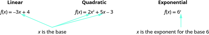
An exponential function, where \(b>0\) and \(b\ne 1\text{,}\) is a function of the form
Notice that in this function, the variable is the exponent. In our functions so far, the variables were the base.
Our definition says \(b\ne 1\text{.}\) If we let \(b=1\text{,}\) then \(f\left(x\right)={b}^{x}\) becomes \(f\left(x\right)={1}^{x}\text{.}\) Since \({1}^{x}=1\) for all real numbers, \(f\left(x\right)={1}^{}\text{.}\) This is the constant function.
Our definition also says \(b>0\text{.}\) If we let a base be negative, say \(-4\text{,}\) then \(f\left(x\right)={\left(-4\right)}^{x}\) is not a real number when \(x=\frac{1}{2}\text{:}\)
In fact, \(f\left(x\right)={\left(-4\right)}^{x}\) would not be a real number any time \(x\) is a fraction with an even denominator. So our definition requires \(b>0\text{.}\)
By graphing a few exponential functions, we will be able to see their unique properties.
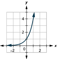
Example 14.1.3.
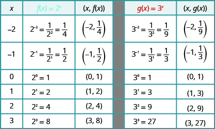
On the same coordinate system graph \(f\left(x\right)={2}^{x}\) and \(g\left(x\right)={3}^{x}\text{.}\)
We will use point plotting to graph the functions.
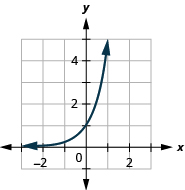
Checkpoint 14.1.6.
Graph: \(f\left(x\right)={4}^{x}\text{.}\)
Checkpoint 14.1.8.
Graph: \(g\left(x\right)={5}^{x}\text{.}\)
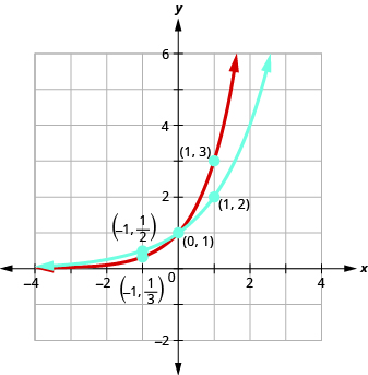
If we look at the graphs from the previous examples, we can identify some of the properties of exponential functions.
The graphs of \(f\left(x\right)={2}^{x}\) and \(g\left(x\right)={3}^{x}\text{,}\) as well as the graphs of \(f\left(x\right)={4}^{x}\) and \(g\left(x\right)={5}^{x}\text{,}\) all have the same basic shape. This is the shape we expect from an exponential function where \(b>1\text{.}\)
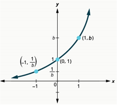
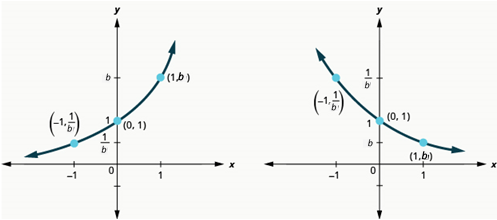
We notice, that for each function, the graph contains the point \(\left(0,1\right)\text{.}\) This makes sense because \({b}^{0}=1\) for any \(b>1\text{.}\)
The graph of each function, \(f\left(x\right)={b}^{x}\) also contains the point \(\left(1,b\right)\text{.}\) The graph of \(f\left(x\right)={2}^{x}\) contains \(\left(1,2\right)\) and the graph of \(g\left(x\right)={3}^{x}\) contains \(\left(1,3\right)\text{.}\) This makes sense as \({b}^{1}=b\) for any \(b>1\text{.}\)
Notice too, that the graph of each function \(f\left(x\right)={b}^{x}\) also contains the point \(\left(-1,\frac{1}{b}\right)\text{.}\) The graph of \(f\left(x\right)={2}^{x}\) contains \(\left(-1,\frac{1}{2}\right)\) and the graph of \(g\left(x\right)={3}^{x}\) contains \(\left(-1,\frac{1}{3}\right)\text{.}\) This makes sense as \({b}^{-1}=\frac{1}{b}\) for any \(b>1\text{.}\)
What is the domain for each function? From the graphs we can see that the domain is the set of all real numbers. There is no restriction on the domain. We write the domain in interval notation as \((-\infty ,\infty)\text{.}\)
Look at each graph. What is the range of the function? Notice that the graph is always above and never touches the \(x\)-axis. Thus, the range is all positive numbers. We write the range in interval notation as \(\left(0,\infty \right)\text{.}\)
Whenever a graph of a function approaches a line but never touches it, we call that line an asymptote. For the exponential functions we are looking at, the graph approaches the \(x\)-axis very closely but will never cross it. So we call the line \(y=0\text{,}\) the \(x\)-axis, a horizontal asymptote.
We summarize these results below.
| Domain | \((-\infty ,\infty)\) |
| Range | \(\left(0,\infty \right)\) |
| \(x\)-intercept | None |
| \(y\)-intercept | \(\left(0,1\right)\) |
| Contains | \(\left(1,b\right), \left(-1,\frac{1}{b}\right)\) |
| Asymptote | \(x\)-axis, the line \(y=0\) |
Our definition of an exponential function \(f\left(x\right)={b}^{x}\) says \(b>0\text{,}\) but the examples and discussion so far has been about functions where \(b>1\text{.}\) What happens when \(0<b<1\text{?}\) The next example will explore this possibility.
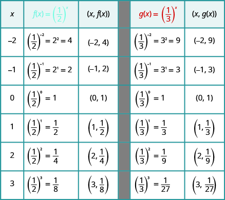
Example 14.1.11.
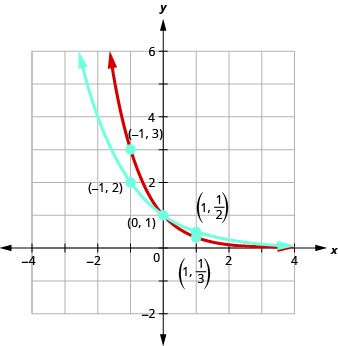
On the same coordinate system, graph \(f\left(x\right)={\left(\frac{1}{2}\right)}^{x}\) and \(g\left(x\right)={\left(\frac{1}{3}\right)}^{x}\text{.}\)
We will use point plotting to graph the functions.
Checkpoint 14.1.14.
Graph: \(f\left(x\right)={\left(\frac{1}{4}\right)}^{x}\text{.}\)
Checkpoint 14.1.16.
Graph: \(g\left(x\right)={\left(\frac{1}{5}\right)}^{x}\text{.}\)
Now let's look at the graphs from the previous examples, so we can now identify some of the properties of exponential functions where \(0<b<1\text{.}\)
The graphs of \(f\left(x\right)={\left(\frac{1}{2}\right)}^{x}\) and \(g\left(x\right)={\left(\frac{1}{3}\right)}^{x}\) as well as the graphs of \(f\left(x\right)={\left(\frac{1}{4}\right)}^{x}\) and \(g\left(x\right)={\left(\frac{1}{5}\right)}^{x}\) all have the same basic shape. While this is the shape we expect from an exponential function, the graphs go down from left to right (i.e. they're decreasing), while the previous graphs, when \(b>1\text{,}\) went from up from left to right (i.e. they're increasing).
We notice that for each function, the graph still contains the point (0, 1). This should make sense because \({b}^{0}=1\) for any \(b>0\text{.}\)
As before, the graph of each function, \(f\left(x\right)={b}^{x}\text{,}\) also contains the point \(\left(1,b\right)\text{.}\) The graph of \(f\left(x\right)={\left(\frac{1}{2}\right)}^{x}\) contains \(\left(1,\frac{1}{2}\right)\) and the graph of \(g\left(x\right)={\left(\frac{1}{3}\right)}^{x}\) contains \(\left(1,\frac{1}{3}\right)\text{.}\) This makes sense as \({b}^{1}=b\) for any \(b\text{.}\)
Notice too that the graph of each function, \(f\left(x\right)={b}^{x}\text{,}\) also contains the point \(\left(-1,\frac{1}{b}\right)\text{.}\) The graph of \(f\left(x\right)={\left(\frac{1}{2}\right)}^{x}\) contains \(\left(-1,2\right)\) and the graph of \(g\left(x\right)={\left(\frac{1}{3}\right)}^{x}\) contains \(\left(-1,3\right)\text{.}\) This makes sense as \({b}^{-1}=\frac{1}{b}\) for any \(b>0\text{.}\)
What is the domain and range for each function? From the graphs we can see that the domain is the set of all real numbers and we write the domain in interval notation as \(\left(-\infty ,\infty \right)\text{.}\) Again, the graph is always above and never touches the \(x\)-axis. Thus, the range is the set of all positive numbers. We write the range in interval notation as \(\left(0,\infty \right)\text{.}\)
We will summarize these properties in Table 14.1.18, which also includes when \(b>1\text{.}\)
| when \(b>1\) | when \(0<b<1\) | ||
| Domain | \(\left(-\infty ,\infty \right)\) | Domain | \(\left(-\infty ,\infty \right)\) |
| Range | \(\left(0,\infty \right)\) | Range | \(\left(0,\infty \right)\) |
| \(x\)-intercept | none | \(x\)-intercept | none |
| \(y\)-intercept | \(\left(0,1\right)\) | \(y\)-intercept | \(\left(0,1\right)\) |
| Contains | \(\left(1,b\right), \left(-1,\frac{1}{b}\right)\) | Contains | \(\left(1,b\right), \left(-1,\frac{1}{b}\right)\) |
| Asymptote | \(x\)-axis, the line \(y=0\) | Asymptote | \(x\)-axis, the line \(y=0\) |
| Basic shape | increasing | Basic shape | decreasing |
Example 14.1.20.
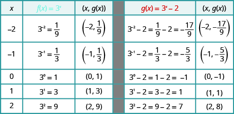
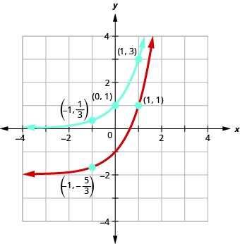
On the same coordinate system, graph \(f\left(x\right)={3}^{x}\) and \(g\left(x\right)={3}^{x}-2\text{.}\)
We will use point plotting to graph the functions.
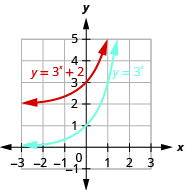
Checkpoint 14.1.23.
On the same coordinate system, graph: \(f\left(x\right)={3}^{x}\) and \(g\left(x\right)={3}^{x}+2\text{.}\)
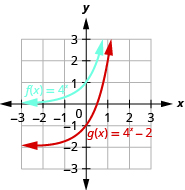
Checkpoint 14.1.25.
On the same coordinate system, graph: \(f\left(x\right)={4}^{x}\) and \(g\left(x\right)={4}^{x}-2\text{.}\)
All of our exponential functions so far have had either an integer or a rational number as the base. We will now look at an exponential function with an irrational number as the base.
Before we can look at this exponential function, we need to define the irrational number, \(e\text{.}\) This number is used as a base in many applications in the sciences and business that are modeled by exponential functions. The number is defined as the value of \({\left(1+\frac{1}{n}\right)}^{n}\) as \(n\) gets larger and larger. We say, as \(n\) approaches infinity, or increases without bound. The table shows the value of \({\left(1+\frac{1}{n}\right)}^{n}\) for several values of \(n\text{.}\)
| \(n\) | \({\left(1+\frac{1}{n}\right)}^{n}\) |
| 1 | 2 |
| 2 | 2.25 |
| 5 | 2.48832 |
| 10 | 2.59374246 |
| 100 | 2.704813829... |
| 1,000 | 2.716923932... |
| 10,000 | 2.718145927... |
| 100,000 | 2.718268237... |
| 1,000,000 | 2.718280469... |
| 1,000,000,000 | 2.718281827... |
The number \(e\) is like the number \(\pi \) in that we use a symbol to represent it because its decimal representation never stops or repeats. The irrational number \(e\) is called the natural base.
Definition 14.1.28. Natural Base e.
The natural base \(e\) is defined as the value of \({\left(1+\frac{1}{n}\right)}^{n}\text{,}\) as \(n\) increases without bound. We say, as \(n\) approaches infinity,
Definition 14.1.29. Natural Exponential Function.
The exponential function whose base is \(e\text{,}\) \(f\left(x\right)={e}^{x}\text{,}\) is called the natural exponential function.
Let's graph the function \(f\left(x\right)={e}^{x}\) on the same coordinate system as \(g\left(x\right)={2}^{x}\) and \(h\left(x\right)={3}^{x}\text{.}\)
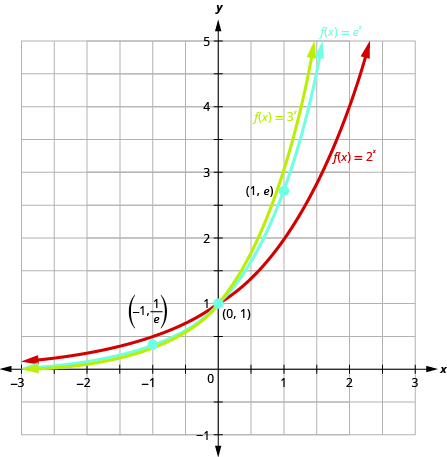
Notice that the graph of \(f\left(x\right)={e}^{x}\) is between the graphs of \(g\left(x\right)={2}^{x}\) and \(h\left(x\right)={3}^{x}\text{.}\) This should make sense as \(2<e<3\text{.}\)
Subsection 14.1.2 Use Exponential Models in Applications
Exponential functions model many situations. If you own a bank account, you have experienced the use of an exponential function, which is used to calculate compound interest. If you've worked in a laboratory with bacteria, then you are familiar with the exponential growth of bacteria, which can be modeled by an exponential function.
Compound Interest.
There are two formulas that are used to determine the balance in the account when interest is earned. If a principal, \(P\text{,}\) is invested at an interest rate, \(r\) (in decimal form), for \(t\) years, the new balance, \(A\text{,}\) will depend on how often the interest is compounded. If the interest is compounded \(n\) times a year we use the formula \(A=P\left(1+\frac{r}{n}\right)^{nt}\text{.}\) If the interest is compounded continuously, we use the formula \(A=P{e}^{rt}\text{.}\) These are the formulas for compound interest.
For a principal, \(P\text{,}\) invested at an interest rate, \(r\) (in decimal form), for \(t\) years, the new balance, \(A\text{,}\) is:
As you work with the interest formulas, it is often helpful to identify the values of the variables first and then substitute them into the formula.
Example 14.1.31.
A total of \(\$10{,}000\) was invested in a college fund for a new grandchild. If the interest rate is \(5\%\text{,}\) how much will be in the account in \(18\) years by each method of compounding?
- compound quarterly
- compound monthly
- compound continuously
| \(A=\text{ ?}\) | |
| Identify the values of each variable in the formulas. | \(P=\$10{,}000\) |
| Be sure to express the percent as a decimal. | \(r=0.05\) |
| \(t=18\) years | |
| a. | |
| For quarterly compounding, \(n=4\) | \(A=P\left(1+\frac{r}{n}\right)^{nt}\) |
| There are \(4\) quarters per year. | |
| Substitute the values in the formula. | \(A=10{,}000\left(1+\frac{0.05}{4}\right)^{4\cdot 18}\) |
| Compute the amount, being careful to follow | |
| the order of operation as you enter the | |
| expression into your calculator. | |
| Round to the nearest cent. | \(A=\$24{,}459.20\) |
| b. | |
| For monthly compounding, \(n=12\) | \(A=P\left(1+\frac{r}{n}\right)^{nt}\) |
| There are \(12\) months per year. | |
| Substitute the values in the formula. | \(A=10{,}000\left(1+\frac{0.05}{12}\right)^{12\cdot 18}\) |
| Compute and round to the nearest cent. | \(A=\$24{,}550.08\) |
| c. | |
| For compounding continuously, | \(A=Pe^{nt}\) |
| Substitute the values in the formula. | \(A=10{,}000e^{0.05\cdot 18}\) |
| Compute and round to the nearest cent. | \(A=\$24{,}596.03\) |
Checkpoint 14.1.33.
Checkpoint 14.1.34.
Exponential Growth and Decay.
Other topics that are modeled by exponential functions involve growth and decay. Both also use the formula \(A=P{e}^{rt}\) we used for the growth of money. For growth and decay, generally we use \({A}_{0}\text{,}\) as the original amount instead of calling it \(P\text{,}\) the principal. We see that exponential growth has a positive rate of growth and exponential decay has a negative rate of growth.
For an original amount, \({A}_{0}\text{,}\) that grows or decays at a rate, \(r\text{,}\) for a certain time, \(t\text{,}\) the final amount, \(A\text{,}\) is:
Exponential growth is typically seen in the growth of populations of humans or animals or bacteria. Our next example looks at the growth of a virus.
Example 14.1.35.
Chris is a researcher at the Center for Disease Control and Prevention and he is trying to understand the behavior of a new and dangerous virus. He starts his experiment with \(100\) of the virus that grows at a rate of \(25\%\) per hour. He will check on the virus in \(24\) hours. How many viruses will he find?
| Identify the values of each variable in the formula. | \(A=\text{ ?}\) |
| Be sure to put the percent in decimal form. | \(A_{0}=100\) |
| Be sure the units match - the rate is per hour, | \(r=0.25\text{/hour}\) |
| the time is in hours. | \(t=24\text{ hours}\) |
| Substitute the values in the formula: \(A=A_{0}e^{rt}\) | \(A=100e^{0.25\cdot 24}\) |
| Compute the amount. | \(A=40,342.88\) |
| Round to the nearest whole virus. | \(A=40,343\) |
| answer the question. | The researcher will find 40,343 viruses. |
Checkpoint 14.1.37.
Checkpoint 14.1.38.
Exercises 14.1.3 Exercises
Evaluate Exponential Functions
1.
For the function \(f(x)= 7^x,\) calculate the following function values:
\(f(-3)=\)
\(f(-1)=\)
\(f(0)=\)
\(f(1)=\)
\(f(3)=\)
2.
For the function \(f(x)= 6^x,\) calculate the following function values:
\(f(-3)=\)
\(f(-1)=\)
\(f(0)=\)
\(f(1)=\)
\(f(3)=\)
3.
For the function \(f(x)= 5^x,\) calculate the following function values:
\(f(-3)=\)
\(f(-1)=\)
\(f(0)=\)
\(f(1)=\)
\(f(3)=\)
4.
For the function \(f(x)= 4^x,\) calculate the following function values:
\(f(-3)=\)
\(f(-1)=\)
\(f(0)=\)
\(f(1)=\)
\(f(3)=\)
Graph Exponential Functions
In the following exercises, graph each exponential function.
5.
\(f(x)=2^x\)
6.
\(g(x)=3^x\)
7.
\(f(x)=6^x\)
8.
\(g(x)=7^x\)
9.
\(f(x)=(1.5)^x\)
10.
\(g(x)=(2.5)^x\)
11.
\(f(x)=\left(\frac{1}{2}\right)^x\)
12.
\(g(x)=\left(\frac{1}{3}\right)^x\)
13.
\(f(x)=\left(\frac{1}{6}\right)^x\)
14.
\(g(x)=\left(\frac{1}{7}\right)^x\)
15.
\(f(x)=(0.4)^x\)
16.
\(g(x)=(0.6)^x\)
In the following exercises, graph each pair of functions in the same coordinate system.
17.
\(f\left(x\right)={4}^{x}, g\left(x\right)={4}^{x-1}\)
18.
\(f\left(x\right)={3}^{x}, g\left(x\right)={3}^{x-1}\)
19.
\(f\left(x\right)={2}^{x}, g\left(x\right)={2}^{x-2}\)
20.
\(f\left(x\right)={2}^{x}, g\left(x\right)={2}^{x+2}\)
21.
\(f\left(x\right)={3}^{x}, g\left(x\right)={3}^{x}+2\)
22.
\(f\left(x\right)={4}^{x}, g\left(x\right)={4}^{x}+2\)
23.
\(f\left(x\right)={2}^{x}, g\left(x\right)={2}^{x}+1\)
24.
\(f\left(x\right)={2}^{x}, g\left(x\right)={2}^{x}-1\)
In the following exercises, graph each exponential function.
25.
\(f\left(x\right)={3}^{x+2}\)
26.
\(f\left(x\right)={3}^{x-2}\)
27.
\(f\left(x\right)={2}^{x}+3\)
28.
\(f\left(x\right)={2}^{x}-3\)
29.
\(f\left(x\right)={\left(\frac{1}{2}\right)}^{x-4}\)
30.
\(f\left(x\right)={\left(\frac{1}{2}\right)}^{x}-3\)
31.
\(f\left(x\right)={e}^{x}+1\)
32.
\(f\left(x\right)={e}^{x-2}\)
33.
\(f\left(x\right)=\text{−}{2}^{x}\)
34.
\(f\left(x\right)={3}^{x}\)
In the following exercises, match the graphs to one of the following functions:
- \(\displaystyle {2}^{x}\)
- \(\displaystyle {2}^{x+1}\)
- \(\displaystyle {2}^{x-1}\)
- \(\displaystyle {2}^{x}+2\)
- \(\displaystyle {2}^{x}-2\)
- \(\displaystyle {3}^{x}\)
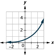
35.
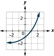
36.
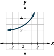
37.
38.
39.
40.
Use Exponential Models in Applications
In the following exercises, use an exponential model to solve.
41.
Edgar accumulated \(\$5,000\) in credit card debt. If the interest rate is \(20\%\) per year, and he does not make any payments for 2 years, how much will he owe on this debt in 2 years by each method of compounding?
compound quarterly:
compound monthly:
compound continuously:
42.
Cynthia invested \(\$12,000\) in a savings account. If the interest rate is \(6\%\text{,}\) how much will be in the account in \(10\) years by each method of compounding?
compound quarterly:
compound monthly:
compound continuously:
43.
Rochelle deposits \(\$5,000\) in an IRA. What will be the value of her investment in \(25\) years if the investment is earning \(8\%\) per year and is compounded continuously?
The value of her investment will be .
44.
Nazerhy deposits \(\$8,000\) in a certificate of deposit. The annual interest rate is \(6\%\) and the interest will be compounded quarterly. How much will the certificate be worth in \(10\) years?
His certificate will be worth .
45.
A researcher at the Center for Disease Control and Prevention is studying the growth of a bacteria. He starts his experiment with \(100\) of the bacteria that grows at a rate of \(6\%\) per hour. He will check on the bacteria every \(8\) hours. How many bacteria will he find in \(8\) hours?
He will find bacteria.
46.
A biologist is observing the growth pattern of a virus. She starts with \(50\) of the virus that grows at a rate of \(20\%\) per hour. She will check on the virus in \(24\) hours. How many viruses will she find?
She will find viruses.
47.
In the last ten years the population of Indonesia has grown at a rate of \(1.12\%\) per year to \(258,316,051\text{.}\) If this rate continues, what will be the population in \(10\) more years?
The population will be .
This section is adapted from "Evaluate and Graph Exponential Functions" 1 by Wendy Lightheart, OpenStax CNX, which is licensed under CC BY 4.0 2 / A derivative from the original work "Evaluate and Graph Exponential Functions" 3 by OpenStax, OpenStax CNX.