Section 4.3 Exploring Two-Variable Data and Rate of Change
This section is about examining data that has been plotted on a Cartesian coordinate system, and then making observations. In some cases, we'll be able to turn those observations into useful mathematical calculations.
Subsection 4.3.1 Modeling data with two variables
Using mathematics, we can analyze real data from the world around us. We can use what we discover to better understand the world, and sometimes to make predictions. Here's an example of data about the economic situation in the US:

If this trend continues, what percentage of all income will the top 1 % have in the year 2030? If we model data in the chart with the trend line, we can estimate the value to be 28.6 %. This is one way math is used in real life.
Does that trend line have an equation like those we looked at in Section 4.2? Is it even correct to look at this data set and decide that a straight line is a good model? These are some of the questions we want to consider as we begin this section. The answers will evolve through the next several sections.
Subsection 4.3.2 Patterns in Tables
Example 4.3.2.
Find a pattern in each table. What is the missing entry in each table? Can you describe each pattern in words and/or mathematics?
| black | white |
| big | small |
| short | tall |
| few |
| USA | Washington |
| UK | London |
| France | Paris |
| Mexico |
| 1 | 2 |
| 2 | 4 |
| 3 | 6 |
| 5 |
| black | white |
| big | small |
| short | tall |
| few | many |
| USA | Washington |
| UK | London |
| France | Paris |
| Mexico | Mexico City |
| 1 | 2 |
| 2 | 4 |
| 3 | 6 |
| 5 | 10 |
- First table
Each word on the right has the opposite meaning of the word to its left.
- Second table
Each city on the right is the capital of the country to its left.
- Third table
Each number on the right is double the number to its left.
We can view each table as assigning each input in the left column a corresponding output in the right column. In the first table, for example, when the input “big” is on the left, the output “small” is on the right.
The first table's function is to output a word with the opposite meaning of each input word. (This is not a numerical example.)
The third table is numerical. And its function is to take a number as input, and give twice that number as its output. Mathematically, we can describe the pattern as “\(y=2x\text{,}\)” where \(x\) represents the input, and \(y\) represents the output. Labeling the table mathematically, we have Table 4.3.5.
| \(x\) (input) |
\(y\) (output) |
| \(1\) | \(2\) |
| \(2\) | \(4\) |
| \(3\) | \(6\) |
| \(5\) | \(10\) |
| \(10\) | \(20\) |
| Pattern: \(y=2x\) | |
The equation \(y=2x\) summarizes the pattern in the table. For each of the following tables, find an equation that describes the pattern you see. Numerical pattern recognition may or may not come naturally for you.
Either way, pattern recognition is an important mathematical skill that anyone can develop. Solutions for these exercises provide some ideas for recognizing patterns.
Checkpoint 4.3.6.
Checkpoint 4.3.7.
Checkpoint 4.3.8.
Subsection 4.3.3 Rate of Change
For an hourly wage-earner, the amount of money they earn depends on how many hours they work. If a worker earns \(\$15\) per hour, then \(10\) hours of work corresponds to \(\$150\) of pay. Working one additional hour will change \(10\) hours to \(11\) hours; and this will cause the \(\$150\) in pay to rise by fifteen dollars to \(\$165\) in pay. Any time we compare how one amount changes (dollars earned) as a consequence of another amount changing (hours worked), we are talking about a rate of change.
Given a table of two-variable data, between any two rows we can compute a rate of change.
Example 4.3.9.
The following data, given in both table and graphed form, gives the counts of invasive cancer diagnoses in Oregon over a period of time. ( wonder.cdc.gov )
| Year | Invasive Cancer Incidents |
| 1999 | 17,599 |
| 2000 | 17,446 |
| 2001 | 17,847 |
| 2002 | 17,887 |
| 2003 | 17,559 |
| 2004 | 18,499 |
| 2005 | 18,682 |
| 2006 | 19,112 |
| 2007 | 19,376 |
| 2008 | 20,370 |
| 2009 | 19,909 |
| 2010 | 19,727 |
| 2011 | 20,636 |
| 2012 | 20,035 |
| 2013 | 20,458 |

What is the rate of change in Oregon invasive cancer diagnoses between 2000 and 2010? The total (net) change in diagnoses over that timespan is
Since \(10\) years passed (which you can calculate as \(2010-2000\)), the rate of change is \(2281\) diagnoses per \(10\) years, or
We read that last quantity as “\(228.1\) diagnoses per year.” This rate of change means that between the years \(2000\) and \(2010\text{,}\) there were \(228.1\) more diagnoses each year, on average. (Notice that there was no single year in that span when diagnoses increased by \(228.1\text{.}\))
Let's practice calculating rates of change over different timespans:
Checkpoint 4.3.10.
We are ready to give a formal definition for rate of change. Considering our work from Example 4.3.9 and Checkpoint 4.3.10, we settle on:
Definition 4.3.11. Rate of Change.
If \(\left(x_1,y_1\right)\) and \(\left(x_2,y_2\right)\) are two data points from a set of two-variable data, then the rate of change between them is
(The Greek letter delta, \(\Delta\text{,}\) is used to represent “change in” since it is the first letter of the Greek word for “difference.” )
In Example 4.3.9 and Checkpoint 4.3.10 we found three rates of change. Figure 4.3.12 highlights the three pairs of points that were used to make these calculations.

Note how the larger the numerical rate of change between two points, the steeper the line is that connects them. This is such an important observation, we'll put it in an official remark.
Remark 4.3.13.
The rate of change between two data points is intimately related to the steepness of the line segment that connects those points.
The steeper the line, the larger the rate of change, and vice versa.
If one rate of change between two data points equals another rate of change between two different data points, then the corresponding line segments will have the same steepness.
When a line segment between two data points slants down from left to right, the rate of change between those points will be negative.
In the solution to Checkpoint 4.3.7, the key observation was that the rate of change from one row to the next was constant: \(3\) units of increase in \(y\) for every \(1\) unit of increase in \(x\text{.}\) Graphing this pattern in Figure 4.3.14, we see that every line segment here has the same steepness, so the entire graph is a line.

Whenever the rate of change is constant no matter which two \((x,y)\)-pairs (or data pairs) are chosen from a data set, then you can conclude the graph will be a straight line even without making the graph. We call this kind of relationship a linear relationship. We'll study linear relationships in more detail throughout this chapter. Right now in this section, we feel it is important to simply identify if data has a linear relationship or not.
Checkpoint 4.3.15.
Checkpoint 4.3.16.
Checkpoint 4.3.17.
Let's return to the data that we opened the section with, in Figure 4.3.1. Is that data linear? Well, yes and no. To be completely honest, it's not linear. It's easy to pick out pairs of points where the steepness changes from one pair to the next. In other words, the points do not all fall into a single line.
However, if we stand back, there does seem to be an overall upward trend that is captured by the line someone has drawn over the data. Points on this line do have a linear pattern. Let's estimate the rate of change between some points on this line. We are free to use any points to do this, so let's make this calculation easier by choosing points we can clearly identify on the graph: \((1991,15)\) and \((2020,25)\text{.}\)

The rate of change between those two points is
So we might say that on average the rate of change expressed by this data is 0.3448 %⁄yr.
Exercises 4.3.4 Exercises
Finding Patterns
1.
Write an equation in the form \(y=\ldots\) suggested by the pattern in the table.
| \(x\) | \(y\) |
| \(-2\) | \({-12}\) |
| \(-1\) | \({-6}\) |
| \(0\) | \({0}\) |
| \(1\) | \({6}\) |
| \(2\) | \({12}\) |
2.
Write an equation in the form \(y=\ldots\) suggested by the pattern in the table.
| \(x\) | \(y\) |
| \(3\) | \({6}\) |
| \(4\) | \({8}\) |
| \(5\) | \({10}\) |
| \(6\) | \({12}\) |
| \(7\) | \({14}\) |
3.
Write an equation in the form \(y=\ldots\) suggested by the pattern in the table.
| \(x\) | \(y\) |
| \(2\) | \({10}\) |
| \(3\) | \({11}\) |
| \(4\) | \({12}\) |
| \(5\) | \({13}\) |
| \(6\) | \({14}\) |
4.
Write an equation in the form \(y=\ldots\) suggested by the pattern in the table.
| \(x\) | \(y\) |
| \(3\) | \({9}\) |
| \(4\) | \({10}\) |
| \(5\) | \({11}\) |
| \(6\) | \({12}\) |
| \(7\) | \({13}\) |
5.
Write an equation in the form \(y=\ldots\) suggested by the pattern in the table.
| \(x\) | \(y\) |
| \(8\) | \({14}\) |
| \(1\) | \({7}\) |
| \(17\) | \({23}\) |
| \(12\) | \({18}\) |
| \(10\) | \({16}\) |
6.
Write an equation in the form \(y=\ldots\) suggested by the pattern in the table.
| \(x\) | \(y\) |
| \(10\) | \({7}\) |
| \(15\) | \({12}\) |
| \(4\) | \({1}\) |
| \(6\) | \({3}\) |
| \(11\) | \({8}\) |
7.
Write an equation in the form \(y=\ldots\) suggested by the pattern in the table.
| \(x\) | \(y\) |
| \(16\) | \({4}\) |
| \(4\) | \({2}\) |
| \(25\) | \({5}\) |
| \(1\) | \({1}\) |
| \(9\) | \({3}\) |
8.
Write an equation in the form \(y=\ldots\) suggested by the pattern in the table.
| \(x\) | \(y\) |
| \(-2\) | \({2}\) |
| \(-5\) | \({5}\) |
| \(-4\) | \({4}\) |
| \(-1\) | \({1}\) |
| \(-2\) | \({2}\) |
9.
Write an equation in the form \(y=\ldots\) suggested by the pattern in the table.
| \(x\) | \(y\) |
| \(0.05\) | \({0.0025}\) |
| \(0.07\) | \({0.0049}\) |
| \(0.09\) | \({0.0081}\) |
| \(0.11\) | \({0.0121}\) |
| \(0.13\) | \({0.0169}\) |
10.
Write an equation in the form \(y=\ldots\) suggested by the pattern in the table.
| \(x\) | \(y\) |
| \(0.02\) | \({0.0004}\) |
| \(0.05\) | \({0.0025}\) |
| \(0.08\) | \({0.0064}\) |
| \(0.11\) | \({0.0121}\) |
| \(0.14\) | \({0.0196}\) |
11.
Write an equation in the form \(y=\ldots\) suggested by the pattern in the table.
| \(x\) | \(y\) |
| \(9\) | \({{\frac{1}{9}}}\) |
| \(2\) | \({{\frac{1}{2}}}\) |
| \(36\) | \({{\frac{1}{36}}}\) |
| \(95\) | \({{\frac{1}{95}}}\) |
| \(47\) | \({{\frac{1}{47}}}\) |
12.
Write an equation in the form \(y=\ldots\) suggested by the pattern in the table.
| \(x\) | \(y\) |
| \(20\) | \({{\frac{1}{20}}}\) |
| \(67\) | \({{\frac{1}{67}}}\) |
| \(76\) | \({{\frac{1}{76}}}\) |
| \(68\) | \({{\frac{1}{68}}}\) |
| \(44\) | \({{\frac{1}{44}}}\) |
Linear Relationships
13.
Does the following table show that \(x\) and \(y\) have a linear relationship?
yes
no
| \(x\) | \(y\) |
| \(0\) | \({39}\) |
| \(1\) | \({43}\) |
| \(2\) | \({47}\) |
| \(3\) | \({51}\) |
| \(4\) | \({55}\) |
| \(5\) | \({59}\) |
14.
Does the following table show that \(x\) and \(y\) have a linear relationship?
yes
no
| \(x\) | \(y\) |
| \(0\) | \({98}\) |
| \(1\) | \({103}\) |
| \(2\) | \({108}\) |
| \(3\) | \({113}\) |
| \(4\) | \({118}\) |
| \(5\) | \({123}\) |
15.
Does the following table show that \(x\) and \(y\) have a linear relationship?
yes
no
| \(x\) | \(y\) |
| \(0\) | \({81}\) |
| \(1\) | \({76}\) |
| \(2\) | \({71}\) |
| \(3\) | \({66}\) |
| \(4\) | \({61}\) |
| \(5\) | \({56}\) |
16.
Does the following table show that \(x\) and \(y\) have a linear relationship?
yes
no
| \(x\) | \(y\) |
| \(4\) | \({48}\) |
| \(5\) | \({44}\) |
| \(6\) | \({40}\) |
| \(7\) | \({36}\) |
| \(8\) | \({32}\) |
| \(9\) | \({28}\) |
17.
Does the following table show that \(x\) and \(y\) have a linear relationship?
yes
no
| \(x\) | \(y\) |
| \(9\) | \({262163}\) |
| \(10\) | \({1.0486\times 10^{6}}\) |
| \(11\) | \({4.19432\times 10^{6}}\) |
| \(12\) | \({1.67772\times 10^{7}}\) |
| \(13\) | \({6.71089\times 10^{7}}\) |
| \(14\) | \({2.68435\times 10^{8}}\) |
18.
Does the following table show that \(x\) and \(y\) have a linear relationship?
yes
no
| \(x\) | \(y\) |
| \(2\) | \({37}\) |
| \(3\) | \({137}\) |
| \(4\) | \({637}\) |
| \(5\) | \({3137}\) |
| \(6\) | \({15637}\) |
| \(7\) | \({78137}\) |
19.
Does the following table show that \(x\) and \(y\) have a linear relationship?
yes
no
| \(x\) | \(y\) |
| \(2\) | \({37}\) |
| \(3\) | \({248}\) |
| \(4\) | \({1029}\) |
| \(5\) | \({3130}\) |
| \(6\) | \({7781}\) |
| \(7\) | \({16812}\) |
20.
Does the following table show that \(x\) and \(y\) have a linear relationship?
yes
no
| \(x\) | \(y\) |
| \(0\) | \({18}\) |
| \(1\) | \({19}\) |
| \(2\) | \({22}\) |
| \(3\) | \({27}\) |
| \(4\) | \({34}\) |
| \(5\) | \({43}\) |
21.
Does the following table show that \(x\) and \(y\) have a linear relationship?
yes
no
| \(x\) | \(y\) |
| \(0\) | \({67.8}\) |
| \(1\) | \({64.7}\) |
| \(2\) | \({61.6}\) |
| \(3\) | \({58.5}\) |
| \(4\) | \({55.4}\) |
| \(5\) | \({52.3}\) |
22.
Does the following table show that \(x\) and \(y\) have a linear relationship?
yes
no
| \(x\) | \(y\) |
| \(9\) | \({25.55}\) |
| \(10\) | \({23.56}\) |
| \(11\) | \({21.57}\) |
| \(12\) | \({19.58}\) |
| \(13\) | \({17.59}\) |
| \(14\) | \({15.6}\) |
23.
Does the following table show that \(x\) and \(y\) have a linear relationship?
yes
no
| \(x\) | \(y\) |
| \(5\) | \({110}\) |
| \(6\) | \({115}\) |
| \(7\) | \({120}\) |
| \(12\) | \({145}\) |
| \(15\) | \({160}\) |
| \(16\) | \({165}\) |
24.
Does the following table show that \(x\) and \(y\) have a linear relationship?
yes
no
| \(x\) | \(y\) |
| \(2\) | \({62}\) |
| \(4\) | \({74}\) |
| \(5\) | \({80}\) |
| \(6\) | \({86}\) |
| \(10\) | \({110}\) |
| \(15\) | \({140}\) |
Calculating Rate of Change
25.
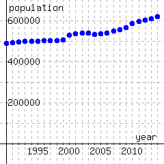
This table gives population estimates for Portland, Oregon from 1990 through 2014.
| Year | Population | Year | Population |
| 1990 | 487849 | 2003 | 539546 |
| 1991 | 491064 | 2004 | 533120 |
| 1992 | 493754 | 2005 | 534112 |
| 1993 | 497432 | 2006 | 538091 |
| 1994 | 497659 | 2007 | 546747 |
| 1995 | 498396 | 2008 | 556442 |
| 1996 | 501646 | 2009 | 566143 |
| 1997 | 503205 | 2010 | 585261 |
| 1998 | 502945 | 2011 | 593859 |
| 1999 | 503637 | 2012 | 602954 |
| 2000 | 529922 | 2013 | 609520 |
| 2001 | 535185 | 2014 | 619360 |
| 2002 | 538803 |
Find the rate of change in Portland population between 1991 and 1993. Just give the numerical value; the units are provided.
\(\,\frac{\text{people}}{\text{year}}\)
And what was the rate of change between 1995 and 2005?
\(\,\frac{\text{people}}{\text{year}}\)
List all the years where there is a negative rate of change between that year and the next year.
26.
This table and graph gives population estimates for Portland, Oregon from 1990 through 2014.
| Year | Population | Year | Population |
| 1990 | 487849 | 2003 | 539546 |
| 1991 | 491064 | 2004 | 533120 |
| 1992 | 493754 | 2005 | 534112 |
| 1993 | 497432 | 2006 | 538091 |
| 1994 | 497659 | 2007 | 546747 |
| 1995 | 498396 | 2008 | 556442 |
| 1996 | 501646 | 2009 | 566143 |
| 1997 | 503205 | 2010 | 585261 |
| 1998 | 502945 | 2011 | 593859 |
| 1999 | 503637 | 2012 | 602954 |
| 2000 | 529922 | 2013 | 609520 |
| 2001 | 535185 | 2014 | 619360 |
| 2002 | 538803 |
Between what two years that are two years apart was the rate of change highest?
What was that rate of change? Just give the numerical value; the units are provided.
\(\,\frac{\text{people}}{\text{year}}\)