
Section 10.1 Function Basics
Subsection 10.1.1 Informal Definition of a Function
In Section 8.1 there is a light introduction to functions. This chapter introduces functions more thoroughly, and is independent from Section 8.1.
We are familiar with the \(\sqrt{\phantom{x}}\) symbol. This symbol is used to turn numbers into their square roots. Sometimes it's simple to do this on paper or in our heads, and sometimes it helps to have a calculator. We can see some calculations in Table 10.1.1.
| \(\sqrt{9}\) | \({}=3\) |
| \(\sqrt{1/4}\) | \({}=1/2\) |
| \(\sqrt{2}\) | \({}\approx1.41\) |
The \(\sqrt{\phantom{x}}\) symbol represents a process; it's a way for us to turn numbers into other numbers. This idea of having a process for turning numbers into other numbers is the fundamental topic of this chapter.
Definition 10.1.2. Function (Informal Definition).
A function is a process for turning numbers into (potentially) different numbers. The process must be consistent, in that whenever you apply it to some particular number, you always get the same result.
Section 10.4 covers a more technical definition for functions, and gets into some topics that are more appropriate when using that definition. Definition 10.1.2 is so broad that you probably use functions all the time.
Example 10.1.3.
Think about each of these examples, where some process is used for turning one number into another.
If you convert a person's birth year into their age, you are using a function.
If you look up the Kelly Blue Book value of a Honda Odyssey based on how old it is, you are using a function.
If you use the expected guest count for a party to determine how many pizzas you should order, you are using a function.
The process of using \(\sqrt{\phantom{x}}\) to change numbers might feel more “mathematical” than these examples. Let's continue thinking about \(\sqrt{\phantom{x}}\) for now, since it's a formula-like symbol that we are familiar with. One concern with \(\sqrt{\phantom{x}}\) is that although we live in the modern age of computers, this symbol is not found on most keyboards. And yet computers still tend to be capable of producing square roots. Computer technicians write \(\operatorname{sqrt}(\phantom{x})\) when they want to compute a square root, as we see in Table 10.1.4.
| \(\operatorname{sqrt}(9)\) | \({}=3\) |
| \(\operatorname{sqrt}(1/4)\) | \({}=1/2\) |
| \(\operatorname{sqrt}(2)\) | \({}\approx1.41\) |
The parentheses are very important. To see why, try to put yourself in the “mind” of a computer, and look closely at sqrt49. The computer will recognize sqrt and know that it needs to compute a square root. But computers have myopic vision and they might not see the entire number \(49\text{.}\) A computer might think that it needs to compute sqrt4 and then append a 9 to the end, which would produce a final result of \(29\text{.}\) This is probably not what was intended. And so the purpose of the parentheses in sqrt(49) is to denote exactly what number needs to be operated on.
This demonstrates the standard notation that is used worldwide to write down most functions. By having a standard notation for communicating about functions, people from all corners of the earth can all communicate mathematics with each other more easily, even when they don't speak the same language.
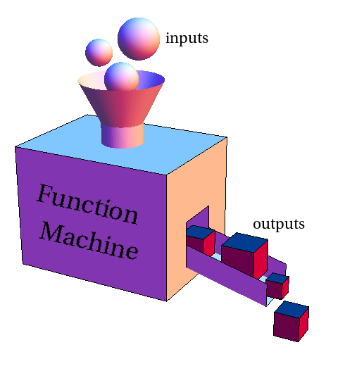
Sometimes it's helpful to think of a function as a machine, as in Figure 10.1.5. This illustrates how complicated functions can be. A number is just a number. But a function has the capacity to take in all kinds of different numbers into it's hopper (feeding tray) as inputs and transform them into their outputs.
Next we need to discuss how we go about using a function's name.
Functions have their own names. We've seen a function named \(\operatorname{sqrt}\text{,}\) but any name you can imagine is allowable. In the sciences, it is common to name functions with whole words, like \(\operatorname{weight}\) or \(\operatorname{health\_index}\text{.}\) In mathematics, we often abbreviate such function names to \(w\) or \(h\text{.}\) And of course, since the word “function” itself starts with “f,” we will often name a function \(f\text{.}\)
It's crucial to continue reminding ourselves that functions are processes for changing numbers; they are not numbers themselves. And that means that we have a potential for confusion that we need to stay aware of. In some contexts, the symbol \(t\) might represent a variable—a number that is represented by a letter. But in other contexts, \(t\) might represent a function—a process for changing numbers into other numbers. By staying conscious of the context of an investigation, we avoid confusion.
Definition 10.1.6. Function Notation.
The standard notation for referring to functions involves giving the function itself a name, and then writing:
Example 10.1.7.
\(f(13)\) is pronounced “f of 13.” The word “of” is very important, because it reminds us that \(f\) is a process and we are about to apply that process to the input value \(13\text{.}\) So \(f\) is the function, \(13\) is the input, and \(f(13)\) is the output we'd get from using \(13\) as input.
\(f(x)\) is pronounced “f of \(x\text{.}\)” This is just like the previous example, except that the input is not any specific number. The value of \(x\) could be \(13\) or any other number. Whatever \(x\)'s value, \(f(x)\) means the corresponding output from the function \(f\text{.}\)
\(\operatorname{BudgetDeficit}(2017)\) is pronounced “BudgetDeficit of 2017.” This is probably about a function that takes a year as input and gives that year's federal budget deficit as output. The process here of changing a year into a dollar amount might not involve any mathematical formula, but rather looking up information from the Congressional Budget Office's website.
\(\operatorname{Celsius}(F)\) is pronounced “Celsius of F.” This is probably about a function that takes a Fahrenheit temperature as input and gives the corresponding Celsius temperature as output. Maybe a formula is used to do this; maybe a chart or some other tool is used to do this. Here, \(\operatorname{Celsius}\) is the function, \(F\) is the input variable, and \(\operatorname{Celsius}(F)\) is the output from the function.
Note 10.1.8.
While a function has a name like \(f\) and the input to that function often has a variable name like \(x\text{,}\) the expression \(f(x)\) represents the output of the function. To be clear, \(f(x)\) is not a function. Rather, \(f\) is a function, and \(f(x)\) its output when the number \(x\) was used as input.
Checkpoint 10.1.9.
Warning 10.1.10. Notation Ambiguity.
As mentioned earlier, we need to remain conscious of the context of any symbol we are using. It's possible for \(f\) to represent a function (a process), but it's also possible for \(f\) to represent a variable (a number). Similarly, parentheses might indicate the input of a function, or they might indicate that two numbers need to be multiplied. It all depends on the context in which these symbols are being used. It's up to our judgment to interpret algebraic expressions in the right context.
Subsection 10.1.2 Tables and Graphs
Since functions are potentially complicated, we want ways to understand them more easily. Two basic tools for understanding a function better are tables and graphs.
Example 10.1.11. A Table for the Budget Deficit Function.
Consider the function \(\operatorname{BudgetDeficit}\text{,}\) that takes a year as its input and outputs the US federal budget deficit for that year. For example, the Congressional Budget Office's website tells us that \(\operatorname{BudgetDeficit}(2009)\) is \(\$1.4\) trillion. If we'd like to understand this function better, we might make a table of all the inputs and outputs we can find. Using the CBO's website ( www.cbo.gov/topics/budget), we can put together Table 10.1.12.
| input \(x\) (year) |
output \(\operatorname{BudgetDeficit}(x)\) (\$trillion) |
| 2007 | \(0.16\) |
| 2008 | \(0.46\) |
| 2009 | \(1.4\) |
| 2010 | \(1.3\) |
| 2011 | \(1.3\) |
| 2012 | \(1.1\) |
| 2013 | \(0.68\) |
| 2014 | \(0.48\) |
| 2015 | \(0.44\) |
| 2016 | \(0.59\) |
How is this table helpful? There are things about the function that we can see now by looking at the numbers in this table.
We can see that the budget deficit had a spike between 2008 and 2009.
And it fell again between 2012 and 2013.
It appears to stay roughly steady for several years at a time, with occasional big jumps or drops.
These observations help us understand the function \(\operatorname{BudgetDeficit}\) a little better.
Checkpoint 10.1.13.
Example 10.1.14. A Table for the Square Root Function.
Let's return to our example of the function \(\operatorname{sqrt}\text{.}\) Tabulating some inputs and outputs reveals Table 10.1.15
| input, \(x\) | output, \(\operatorname{sqrt}(x)\) |
| \(0\) | \(0\) |
| \(1\) | \(1\) |
| \(2\) | \(\approx1.41\) |
| \(3\) | \(\approx1.73\) |
| \(4\) | \(2\) |
| \(5\) | \(\approx2.24\) |
| \(6\) | \(\approx2.45\) |
| \(7\) | \(\approx2.65\) |
| \(8\) | \(\approx2.83\) |
| \(9\) | \(3\) |
How is this table helpful? Here are some observations that we can make now.
We can see that when input numbers increase, so do output numbers.
We can see even though outputs are increasing, they increase by less and less with each step forward in \(x\text{.}\)
These observations help us understand \(\operatorname{sqrt}\) a little better. For instance, based on these observations, which do you think is larger: the difference between \(\operatorname{sqrt}(23)\) and \(\operatorname{sqrt}(24)\text{,}\) or the difference between \(\operatorname{sqrt}(85)\) and \(\operatorname{sqrt}(86)\text{?}\)
Checkpoint 10.1.16.
Another powerful tool for understanding functions better is a graph. Given a function \(f\text{,}\) one way to make its graph is to take a table of input and output values, and read each row as the coordinates of a point in the \(xy\)-plane.
Example 10.1.17. A Graph for the Budget Deficit Function.
Returning to the function \(\operatorname{BudgetDeficit}\) that we studied in Example 10.1.11, in order to make a graph of this function we view Table 10.1.12 as a list of points with \(x\) and \(y\) coordinates, as in Table 10.1.18. We then plot these points on a set of coordinate axes, as in Figure 10.1.19. The points have been connected with a curve so that we can see the overall pattern given by the progression of points. Since there was not any actual data for inputs in between any two years, the curve is dashed. That is, this curve is dashed because it just represents someone's best guess as to how to connect the plotted points. Only the plotted points themselves are precise.
| \((\text{input},\text{output})\) \((x,\operatorname{BudgetDeficit}(x))\) |
| \((2007,0.16)\) |
| \((2008,0.46)\) |
| \((2009,1.4)\) |
| \((2010,1.3)\) |
| \((2011,1.3)\) |
| \((2012,1.1)\) |
| \((2013,0.68)\) |
| \((2014,0.48)\) |
| \((2015,0.44)\) |
| \((2016,0.59)\) |

How has this graph helped us to understand the function better? All of the observations that we made in Example 10.1.11 are perhaps even more clear now. For instance, the spike in the deficit between 2008 and 2009 is now visually apparent. Seeking an explanation for this spike, we recall that there was a financial crisis in late 2008. Revenue from income taxes dropped at the same time that federal money was spent to prevent further losses.
Example 10.1.20. A Graph for the Square Root Function.
Let's now construct a graph for \(\operatorname{sqrt}\text{.}\) Tabulating inputs and outputs gives the points in Table 10.1.21, which in turn gives us the graph in Figure 10.1.22.
| \((\text{input},\text{output})\) \((x,\operatorname{sqrt}(x))\) |
| \((0,0)\) |
| \((1,1)\) |
| \(\approx(2,1.41)\) |
| \(\approx(3,1.73)\) |
| \((4,2)\) |
| \(\approx(5,2.24)\) |
| \(\approx(6,2.45)\) |
| \(\approx(7,2.65)\) |
| \(\approx(8,2.83)\) |
| \((9,3)\) |

Just as in the previous example, we've plotted points where we have concrete coordinates, and then we have made our best attempt to connect those points with a curve. Unlike the previous example, here we believe that points will continue to follow the same pattern indefinitely to the right, and so we have added an arrowhead to the graph.
What has this graph done to improve our understanding of \(\operatorname{sqrt}\text{?}\) As inputs (\(x\)-values) increase, the outputs (\(y\)-values) increase too, although not at the same rate. In fact, we can see that our graph is steep on its left, and less steep as we move to the right. This confirms our earlier observation in Example 10.1.14 that outputs increase by smaller and smaller amounts as the input increases.
Note 10.1.23. Graph of a Function.
Given a function \(f\text{,}\) when we refer to a graph of \(f\) we are not referring to an entire picture, like Figure 10.1.22. A graph of \(f\) is only part of that picture—the curve and the points that it connects. Everything else: axes, tick marks, the grid, labels, and the surrounding white space is just useful decoration, so that we can read the graph more easily.
It is also common to refer to the graph of \(f\) as the graph of the equation \(y=f(x)\). However, we should avoid saying “the graph of \(f(x)\text{.}\)” That would indicate a fundamental misunderstanding of our notation. We have decided that \(f(x)\) is the output for a certain input \(x\text{.}\) That means that \(f(x)\) is just a number; a relatively uninteresting thing compared to \(f\) the function, and not worthy of a two-dimensional picture.
While it is important to be able to make a graph of a function \(f\text{,}\) we also need to be capable of looking at a graph and reading it well. A graph of \(f\) provides us with helpful specific information about \(f\text{;}\) it tells us what \(f\) does to its input values. When we were making graphs, we plotted points of the form
Now given a graph of \(f\text{,}\) we interpret coordinates in the same way.
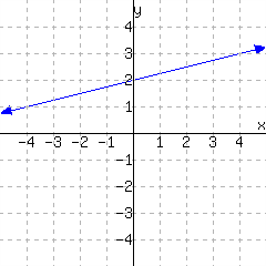
Example 10.1.24.
Below we have a graph of a function \(f\text{.}\) If we wish to find \(f(1)\text{,}\) we recognize that \(1\) is being used as an input. So we would want to find a point of the form \((1,\phantom{y})\text{.}\) Seeking out \(x\)-coordinate \(1\) in Figure 10.1.25, we find that the only such point is \((1,2)\text{.}\) Therefore, the output for \(1\) is \(2\text{;}\) in other words \(f(1)=2\text{.}\)

Checkpoint 10.1.26.
Example 10.1.27. Unemployment Rates.
Suppose that \(u\) is the unemployment function of time. That is, \(u(t)\) is the unemployment rate in the United States in year \(t\text{.}\) The graph of the equation \(y=u(t)\) is given in Figure 10.1.28 ( data.bls.gov/timeseries/LNS14000000).

What was the unemployment in 2008? It is a straightforward matter to use Figure 10.1.28 to find that unemployment was about \(6\%\) in 2008. Asking this question is exactly the same thing as asking to find \(u(2008)\text{.}\) That is, we have one question that can either be asked in an everyday-English way or which can be asked in a terse, mathematical notation-heavy way:
“What was unemployment in 2008?”
“Find \(u(2008)\text{.}\)”
If we use the table to establish that \(u(2009)\approx9.25\text{,}\) then we should be prepared to translate that into everyday-English using the context of the function: In 2009, unemployment in the U.S. was about \(9.25\%\text{.}\)
Checkpoint 10.1.29.
Subsection 10.1.3 Translating Between Four Descriptions of the Same Function
We have noted that functions are complicated, and we want ways to make them easier to understand. It's common to find a problem involving a function and not know how to find a solution to that problem. Most functions have at least four standard ways to think about them, and if we learn how to translate between these four perspectives, we often find that one of them makes a given problem easier to solve.
The four modes for working with a given function are
a verbal description
a table of inputs and outputs
a graph of the function
a formula for the function
This has been visualized in Figure 10.1.30.

Example 10.1.31.
Consider a function \(f\) that squares its input and then adds \(1\text{.}\) Translate this verbal description of \(f\) into a table, a graph, and a formula.
To make a table for \(f\text{,}\) we'll have to select some input \(x\)-values. These choices are left entirely up to us, so we might as well choose small, easy-to-work-with values. However, we shouldn't shy away from negative input values. Given the verbal description, we should be able to compute a column of output values. Table 10.1.32 is one possible table that we might end up with.
| \(x\) | \(f(x)\) |
| \(-2\) | \((-2)^2+1=5\) |
| \(-1\) | \((-1)^2+1=2\) |
| \(0 \) | \(0^2+1=1\) |
| \(1 \) | \(1^2+1=2\) |
| \(2 \) | \(5\) |
| \(3 \) | \(10\) |
| \(4 \) | \(17\) |
Once we have a table for \(f\text{,}\) we can make a graph for \(f\) as in Figure 10.1.33, using the table to plot points.

Lastly, we must find a formula for \(f\text{.}\) This means we need to write an algebraic expression that says the same thing about \(f\) as the verbal description, the table, and the graph. For this example, we can focus on the verbal description. Since \(f\) takes its input, squares it, and adds \(1\text{,}\) we have that
Example 10.1.34.
Let \(F\) be the function that takes a Celsius temperature as input and outputs the corresponding Fahrenheit temperature. Translate this verbal description of \(F\) into a table, a graph, and a formula.
To make a table for \(F\text{,}\) we will need to rely on what we know about Celsius and Fahrenheit temperatures. It is a fact that the freezing temperature of water at sea level is 0 °C, which equals 32 °F. Also, the boiling temperature of water at sea level is 100 °C, which is the same as 212 °F. One more piece of information we might have is that standard human body temperature is 37 °C, or 98.6 °F. All of this is compiled in Table 10.1.35.
Note that we tabulated inputs and outputs by working with the context of the function, not with any computations.
| \(C\) | \(F(C)\) |
| \(0 \) | \(32\) |
| \(37 \) | \(98.6\) |
| \(100 \) | \(212\) |
Once a table is established, making a graph by plotting points is a simple matter, as in Figure 10.1.36. The three plotted points seem to be in a straight line, so we think it is reasonable to connect them in that way.

To find a formula for \(F\text{,}\) the verbal definition is not of much direct help. But \(F\)'s graph does seem to be a straight line. And linear equations are familiar to us. This line has a \(y\)-intercept at \((0,32)\) and a slope we can calculate: \(\frac{212-32}{100-0}=\frac{180}{100}=\frac{9}{5}\text{.}\) So the equation of this line is \(y=\frac{9}{5}C+32\text{.}\) On the other hand, the equation of this graph is \(y=F(C)\text{,}\) since it is a graph of the function \(F\text{.}\) So evidently,
Subsection 10.1.4 Evaluating Functions and Solving Equations That Have Function Notation
Evaluating a function and solving an equation that has function notation in it are two separate things. Students understandably mix up these two tasks, because they are two sides of the same coin. Evaluating a function means that you know an input (typically, an \(x\)-value) and then you calculate an output (typically, a \(y\)-value). Solving an equation that has function notation in it is the opposite process. You know an output (typically, a \(y\)-value) and then you determine all the inputs that could have led to that output (typically, \(x\)-values).
Example 10.1.37.
Evaluate the function \(f\text{,}\) for each of the given values, where \(f(x)=9-5x\text{.}\)
\(\displaystyle f(-2)\)
\(\displaystyle f(0)\)
\(\displaystyle f(4)\)
-
We find \(f(-2)\) by replacing all the \(x\)'s in the formula for \(f\) with \(-2\) and then simplifying the expression as much as possible.
\begin{align*} f(\substitute{-2}) \amp= 9-5(\substitute{-2})\\ \amp= 9+10\\ \amp= 19 \end{align*}Therefore, \(f(-2)=19\)
-
We find \(f(0)\) by replacing all the \(x\)'s in the formula for \(f\) with \(0\) and then simplifying the expression as much as possible.
\begin{align*} f(\substitute{0}) \amp= 9-5(\substitute{0})\\ \amp= 9-0\\ \amp= 9 \end{align*}Therefore, \(f(0)=9\)
-
We find \(f(4)\) by replacing all the \(x\)'s in the formula for \(f\) with \(4\) and then simplifying the expression as much as possible.
\begin{align*} f(\substitute{4}) \amp= 9-5(\substitute{4})\\ \amp= 9-20\\ \amp= -11 \end{align*}Therefore, \(f(4)=-11\)
Checkpoint 10.1.38. Evaluating a Function.
In Example 10.1.37 and Checkpoint 10.1.38, we found the output value of a function when given the input value. This process we refer to as evaluating a function. In contrast, to solve an equation that has function notation in it, we need to solve for the value of the variable that makes an equation true, just like in any other equation. Thus, we need to find the input value(s) that will result in the given output value when the function is applied. This process will be demonstrated in the following example.
Example 10.1.39.
Solve the equations below for a function \(f\) where \(f(x)=8x-9\text{.}\) Check each answer and state the solution set.
\(\displaystyle f(x)=-1\)
\(\displaystyle f(x)=0\)
\(\displaystyle f(x)=15\)
-
To solve for \(x\text{,}\) we will substitute \(f(x)\) with its formula, \(8x-9\text{,}\) and then solve for \(x\text{:}\)
\begin{align*} f(x) \amp= -1\\ \substitute{8x-9} \amp= -1\\ 8x \amp= 8\\ x \amp=1 \end{align*}To check, verify that \(f(1)=-1\text{:}\)
\begin{align*} f(1) \amp= 8(1)-9\\ \amp= 8-9\\ \amp\stackrel{\checkmark}{=} -1 \end{align*}The solution is \(1\text{,}\) and the solution set is \(\{1\}\text{.}\)
-
To solve for \(x\text{,}\) we will substitute \(f(x)\) with its formula, and then solve for \(x\text{:}\)
\begin{align*} f(x) \amp= 0\\ \substitute{8x-9} \amp= 0\\ 8x \amp= 9\\ x \amp=\frac{9}{8} \end{align*}To check, we will verify that \(f\mathopen{}\left(\frac{9}{8}\right)\mathclose{}=0\text{:}\)
\begin{align*} f\mathopen{}\left(\frac{9}{8}\right)\mathclose{} \amp = 8\left(\frac{9}{8}\right)-9\\ \amp= 9-9\\ \amp\stackrel{\checkmark}{=} 0 \end{align*}The solution is \(\frac{9}{8}\text{,}\) and the solution set is \(\left\{\frac{9}{8}\right\}\text{.}\)
-
To solve for \(x\text{,}\) we will substitute \(f(x)\) with its formula, and then solve for \(x\text{:}\)
\begin{align*} f(x) \amp= 15\\ \substitute{8x-9} \amp= 15\\ 8x \amp= 24\\ x \amp= 3 \end{align*}To check, we will verify that \(f(3)=15\text{:}\)
\begin{align*} f(3) \amp= 8(3)-9\\ \amp= 24-9\\ \amp\stackrel{\checkmark}{=} 15 \end{align*}The solution is \(3\text{,}\) and the solution set is \(\{3\}\text{.}\)
Checkpoint 10.1.40.
Subsection 10.1.5 Solving Equations Using Tables or Graphs
Example 10.1.41.
In Checkpoint 10.1.13, we evaluated a function given in table form, using Table 10.1.12. Let's use that same function to solve equations.
Solve \(\text{BudgetDeficit}(x)=0.48\text{.}\) Explain what this solution set represents in context.
Solve \(\text{BudgetDeficit}(x)=1.3\text{.}\) Explain what this solution set represents in context.
To solve \(\text{BudgetDeficit}(x)=0.48\text{,}\) we need to find the value(s) of \(x\) that makes the equation true. Looking at the table, we look at the outputs and see that the output \(0.48\) occurs when \(x=2014\text{.}\) In abstract terms, the solution set is \(\{2014\}\text{.}\) In context, this means that the US federal budget deficit was \(\$0.48\) trillion (or \(\$480\) billion) in 2014.
To solve \(\text{BudgetDeficit}(x)=1.3\text{,}\) we need to find the value(s) of \(x\) that makes the equation true. Looking at the table, we look at the outputs and see that the output \(1.3\) occurs when \(x=2010\) and again when \(x=2011\text{.}\) In abstract terms, the solution set is \(\{2010,2011\}\text{.}\) In context, this means that the US federal budget deficit was \(\$1.3\) trillion in 2010 and again in 2011.
A function may be described using a graph, where the horizontal axis corresponds to possible input values (the domain), and the vertical axis corresponds to possible output values (the range).
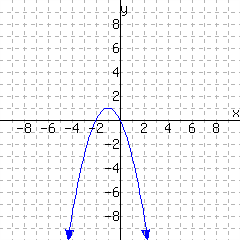
Example 10.1.42.
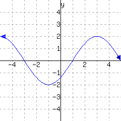
In Example 10.1.24, we evaluated a function given in graphical form, using Figure 10.1.25. Now let's use that same function to solve some equations.
Solve \(f(x)=3\text{.}\)
Solve \(f(x)=2\text{.}\)
-
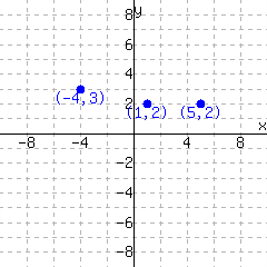
To solve \(f(x)=3\text{,}\) we need to consider the number \(3\) as an output value, so it belongs on the vertical axis in Figure 10.1.43. Moving straight right or left, we find the points \((2,3)\) and \((3,3)\) are on the graph, and that tells us that \(f(x)=3\) when \(x=2\) and when \(x=3\text{.}\) Thus, the solution set is \(\{2,3\}\text{.}\)

Figure 10.1.43. \(y=f(x)\) -
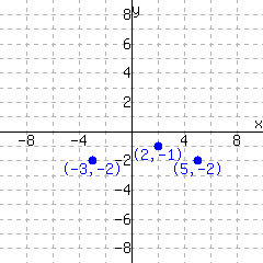
To solve \(f(x)=2\text{,}\) we need to consider the number \(2\) as an output value, so it belongs on the vertical axis in Figure 10.1.44. Moving straight right or left, we find the points \((1,2)\) and \((4,2)\) are on the graph, and that tells us that \(f(x)=2\) when \(x=1\) and when \(x=4\text{.}\) Thus, the solution set is \(\{1,4\}\text{.}\)

Figure 10.1.44. \(y=f(x)\)
Exercises 10.1.6 Exercises
Review and Warmup
1.
Evaluate \(\displaystyle{{\frac{4r-4}{2r}}}\) for \(r=-9\text{.}\)
2.
Evaluate \(\displaystyle{{\frac{7t-7}{2t}}}\) for \(t=5\text{.}\)
3.
Evaluate \({3t^{2}}\) when \(t=2\text{.}\)
Evaluate \({\left(3t\right)^{2}}\) when \(t=2\text{.}\)
4.
Evaluate \({2x^{2}}\) when \(x=3\text{.}\)
Evaluate \({\left(2x\right)^{2}}\) when \(x=3\text{.}\)
5.
Locate each point in the graph:
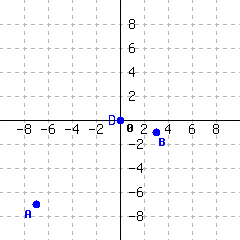
Write each point’s position as an ordered pair, like \((1,2)\text{.}\)
| \(A=\) | \(B=\) |
| \(C=\) | \(D=\) |
6.
Locate each point in the graph:
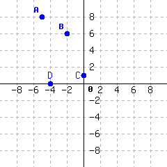
Write each point’s position as an ordered pair, like \((1,2)\text{.}\)
| \(A=\) | \(B=\) |
| \(C=\) | \(D=\) |
Function Formulas and Evaluation
7.
Evaluate the function at the given values.
\(f(x)={x-3}\)
\(f(1)=\)
\(f(-2)=\)
\(f(0)=\)
8.
Evaluate the function at the given values.
\(H(x)={x-1}\)
\(H(4)=\)
\(H(-5)=\)
\(H(0)=\)
9.
Evaluate the function at the given values.
\(F(x)={4x}\)
\(F(3)=\)
\(F(-3)=\)
\(F(0)=\)
10.
Evaluate the function at the given values.
\(G(x)={10x}\)
\(G(5)=\)
\(G(-5)=\)
\(G(0)=\)
11.
Evaluate the function at the given values.
\(H(x)={-3x+5}\)
\(H(5)=\)
\(H(-1)=\)
\(H(0)=\)
12.
Evaluate the function at the given values.
\(K(x)={-4x+9}\)
\(K(4)=\)
\(K(-1)=\)
\(K(0)=\)
13.
Evaluate the function at the given values.
\(f(x)={-x+10}\)
\(f(2)=\)
\(f(-4)=\)
\(f(0)=\)
14.
Evaluate the function at the given values.
\(f(x)={-x+6}\)
\(f(4)=\)
\(f(-5)=\)
\(f(0)=\)
15.
Evaluate the function at the given values.
\(g(x)={x^{2}-9}\)
\(g(4)=\)
\(g(-1)=\)
\(g(0)=\)
16.
Evaluate the function at the given values.
\(h(t)={t^{2}+9}\)
\(h(5)=\)
\(h(-3)=\)
\(h(0)=\)
17.
Evaluate the function at the given values.
\(F(r)={-r^{2}+9}\)
\(F(2)=\)
\(F(-1)=\)
\(F(0)=\)
18.
Evaluate the function at the given values.
\(F(x)={-x^{2}-4}\)
\(F(5)=\)
\(F(-1)=\)
\(F(0)=\)
19.
Evaluate the function at the given values.
\(G(t)={5}\)
\(G(4)=\)
\(G(5)=\)
\(G(0)=\)
20.
Evaluate the function at the given values.
\(H(y)={-7}\)
\(H(3)=\)
\(H(-7)=\)
\(H(0)=\)
21.
Evaluate the function at the given values.
\(\displaystyle{K(x)=\frac{{3x}}{{2x-8}}}\)
\(K(7)=\) .
\(K(-5)=\) .
22.
Evaluate the function at the given values.
\(\displaystyle{K(x)=\frac{{7x}}{{10x+8}}}\)
\(K(7)=\) .
\(K(-1)=\) .
23.
Evaluate the function at the given values.
\(\displaystyle{f(x)={\frac{2}{x+2}}}\) .
\(\displaystyle{f(-4)=}\) .
\(\displaystyle{f(-2)=}\) .
24.
Evaluate the function at the given values.
\(\displaystyle{g(x)={-\frac{63}{x-4}}}\) .
\(\displaystyle{g(11)=}\) .
\(\displaystyle{g(4)=}\) .
25.
Evaluate the function at the given values.
\(\displaystyle{ h(x)={-3x-4} }\)
\(\displaystyle{ h(1)= }\)
\(\displaystyle{ h(-2)= }\)
26.
Evaluate the function at the given values.
\(\displaystyle{ F(x)={-5x+3} }\)
\(\displaystyle{ F(6)= }\)
\(\displaystyle{ F(-2)= }\)
27.
Evaluate the function at the given values.
\(F(x)={x^{2}-5x-5}\)
\(F(2)=\)
\(F(-2)=\)
28.
Evaluate the function at the given values.
\(G(x)={x^{2}+2x}\)
\(G(1)=\)
\(G(-2)=\)
29.
Evaluate the function at the given values.
\(H(x)={-3x^{2}+5x+5}\)
\(H(4)=\)
\(H(-4)=\)
30.
Evaluate the function at the given values.
\(K(x)={-3x^{2}-2x+2}\)
\(K(4)=\)
\(K(-1)=\)
31.
Evaluate the function at the given values.
\(K(x)={\sqrt{x}}\text{.}\)
\(K(49)=\)
\(K\left({{\frac{64}{25}}}\right)=\)
\(K(-3)=\)
32.
Evaluate the function at the given values.
\(f(x)={\sqrt{x}}\text{.}\)
\(f(16)=\)
\(f\left({{\frac{4}{81}}}\right)=\)
\(f(-3)=\)
33.
Evaluate the function at the given values.
\(g(x)=\sqrt[3]{x}\)
\(g(-1)=\)
\(g\left({{\frac{27}{125}}}\right)=\)
34.
Evaluate the function at the given values.
\(h(x)=\sqrt[3]{x}\)
\(h(-8)=\)
\(h\left({{\frac{125}{64}}}\right)=\)
35.
Evaluate the function at the given values.
\(\displaystyle{F(x)={-10}}\)
\(F(4)=\)
\(F(-6)=\)
36.
Evaluate the function at the given values.
\(\displaystyle{F(x)={17}}\)
\(F(7)=\)
\(F(-1)=\)
Function Formulas and Solving Equations
37.
Solve for \(x\text{,}\) where \(G(x)={8x-4}\text{.}\)
\(G(x)={-20}\)
\(G(x)={2}\)
38.
Solve for \(x\text{,}\) where \(H(x)={-8x+7}\text{.}\)
\(H(x)={15}\)
\(H(x)={-5}\)
39.
Solve for \(x\text{,}\) where \(K(x)={x^{2}+8}\text{.}\)
\(K(x)={9}\)
\(K(x)=-1\)
40.
Solve for \(x\text{,}\) where \(K(x)={x^{2}+1}\text{.}\)
\(K(x)={10}\)
\(K(x)=-1\)
41.
Solve for \(x\text{,}\) where \(f(x)={x^{2}+2x-61}\text{.}\)
\(f(x)=2\)
42.
Solve for \(x\text{,}\) where \(g(x)={x^{2}+3x-32}\text{.}\)
\(g(x)=-4\)
43.
If \(F\) is a function defined by \(F(y) = {4y-11}\text{,}\)
Find \(F(0)\text{.}\)
Solve \(F(y)=0\text{.}\)
44.
If \(f\) is a function defined by \(f(y) = {-5y+6}\text{,}\)
Find \(f(0)\text{.}\)
Solve \(f(y)=0\text{.}\)
45.
If \(H\) is a function defined by \(H(r) = {3r^{2}-6}\text{,}\)
Find \(H(0)\text{.}\)
Solve \(H(r)=0\text{.}\)
46.
If \(F\) is a function defined by \(F(r) = {r^{2}-3}\text{,}\)
Find \(F(0)\text{.}\)
Solve \(F(r)=0\text{.}\)
47.
If \(f\) is a function defined by \(f(t) = {t^{2}-13t+30}\text{,}\)
Find \(f(0)\text{.}\)
Solve \(f(t)=0\text{.}\)
48.
If \(H\) is a function defined by \(H(t) = {t^{2}-9t+20}\text{,}\)
Find \(H(0)\text{.}\)
Solve \(H(t)=0\text{.}\)
Solving Equations with Function Notation
49.
Solve for \(x\text{,}\) where \(K(x)={-9x-2}\text{.}\)
\(K(x)={-11}\)
\(K(x)={13}\)
50.
Solve for \(x\text{,}\) where \(f(x)={6x+8}\text{.}\)
\(f(x)={-16}\)
\(f(x)={28}\)
51.
Solve for \(x\text{,}\) where \(g(x)={x^{2}+4}\text{.}\)
\(g(x)={5}\)
\(g(x)=2\)
52.
Solve for \(x\text{,}\) where \(h(x)={x^{2}-3}\text{.}\)
\(h(x)={6}\)
\(h(x)=-8\)
53.
Solve for \(x\text{,}\) where \(F(x)={x^{2}-x-95}\text{.}\)
\(F(x)=-5\)
54.
Solve for \(x\text{,}\) where \(F(x)={x^{2}+9x-4}\text{.}\)
\(F(x)=6\)
Functions and Points on a Graph
55.
If \(G(4)=7\text{,}\) then the point is on the graph of \(G\text{.}\)
If \({\left(8,7\right)}\) is on the graph of \(G\text{,}\) then \(G(8)=\).
56.
If \(H(10)=6\text{,}\) then the point is on the graph of \(H\text{.}\)
If \({\left(5,4\right)}\) is on the graph of \(H\text{,}\) then \(H(5)=\).
57.
If \({\left(r,x\right)}\) is on the graph of \(K\text{,}\) then \(K(r)=\).
58.
If \({\left(y,x\right)}\) is on the graph of \(K\text{,}\) then \(K(y)=\).
59.
For the function \(f\text{,}\) when \(x=1\text{,}\) the output is \({4}\text{.}\)
Choose all true statements.
The function's value is \(1\) at \(4\text{.}\)
The function's value is \(4\) at \(1\text{.}\)
The point \((1, 4)\) is on the graph of the function.
The point \((4, 1)\) is on the graph of the function.
\(\displaystyle f(1)=4\)
\(\displaystyle f(4)=1\)
60.
For the function \(g\text{,}\) when \(x=-2\text{,}\) the output is \({2}\text{.}\)
Choose all true statements.
The function's value is \(-2\) at \(2\text{.}\)
\(\displaystyle g(-2)=2\)
The point \((-2, 2)\) is on the graph of the function.
\(\displaystyle g(2)=-2\)
The function's value is \(2\) at \(-2\text{.}\)
The point \((2, -2)\) is on the graph of the function.
Function Graphs
61.
Use the graph of \(h\) below to evaluate the given expressions. (Estimates are OK.)
\(h(-2)={}\)
\(h(1)={}\)
62.
Use the graph of \(h\) below to evaluate the given expressions. (Estimates are OK.)
\(h(-2)={}\)
\(h(3)={}\)
63.
Use the graph of \(F\) below to evaluate the given expressions. (Estimates are OK.)
\(F(-1)={}\)
\(F(1)={}\)
64.
Use the graph of \(G\) below to evaluate the given expressions. (Estimates are OK.)
\(G(-3)={}\)
\(G(6)={}\)
65.
Use the graph of \(H\) below to evaluate the given expressions. (Estimates are OK.)
\(H(1)={}\)
\(H(5)={}\)
66.
Use the graph of \(K\) below to evaluate the given expressions. (Estimates are OK.)
\(K(-2)={}\)
\(K(2)={}\)
67.
Function \(f\) is graphed.
Find \(\displaystyle{f(2)}\text{.}\)
Solve \(\displaystyle{f(x)=-2}\text{.}\)
68.
Function \(f\) is graphed.
Find \(\displaystyle{f(-4)}\text{.}\)
Solve \(\displaystyle{f(x)=2}\text{.}\)
69.
Function \(f\) is graphed.
Find \(\displaystyle{f(-2)={}}\text{.}\)
Solve \(\displaystyle{f(x)=2}\text{.}\)
70.
Function \(f\) is graphed.
Find \(\displaystyle{f(-1)={}}\text{.}\)
Solve \(\displaystyle{f(x)=0}\text{.}\)
71.
Function \(f\) is graphed.
Find \(\displaystyle{f(0)={}}\text{.}\)
Solve \(\displaystyle{f(x)=-1}\text{.}\)
72.
Function \(f\) is graphed.
Find \(\displaystyle{f(1)={}}\text{.}\)
Solve \(\displaystyle{f(x)=1}\text{.}\)
Function Tables
73.
Use the table of values for \(G\) below to evaluate the given expressions.
| \(x\) | \(-1\) | \(0\) | \(1\) | \(2\) | \(3\) |
| \(G(x)\) | \(6.7\) | \(0.2\) | \(0.5\) | \(4.5\) | \(2.6\) |
\(G({1})={}\)
\(G({3})={}\)
74.
Use the table of values for \(H\) below to evaluate the given expressions.
| \(x\) | \(-1\) | \(3\) | \(7\) | \(11\) | \(15\) |
| \(H(x)\) | \(3.4\) | \(0\) | \(6.6\) | \(5.6\) | \(7.5\) |
\(H({7})={}\)
\(H({11})={}\)
75.
Make a table of values for the function \(H\text{,}\) defined by \(H(x)={4x^{2}}\text{.}\) Based on values in the table, sketch a graph of \(H\text{.}\)
| \(x\) | \(H(x)\) |
76.
Make a table of values for the function \(h\text{,}\) defined by \(\displaystyle h(x)={\frac{2^{x}+5}{x^{2}+2}}\text{.}\) Based on values in the table, sketch a graph of \(h\text{.}\)
| \(x\) | \(h(x)\) |
Translating Between Different Representations of a Function
77.
Here is a verbal description of a function \(f\text{.}\)
“Cube the input \(x\) to obtain the output \(y\text{.}\)”
-
Give a numeric representation of \(f\text{.}\)
\(x\) \(0\) \(1\) \(2\) \(3\) \(4\) \(f(x)\) Give a formula for \(f\text{.}\)
78.
Here is a verbal description of a function \(g\text{.}\)
“Square the input \(x\) to obtain the output \(y\text{.}\)”
-
Give a numeric representation of \(g\text{.}\)
\(x\) \(0\) \(1\) \(2\) \(3\) \(4\) \(g(x)\) Give a formula for \(g\text{.}\)
79.
Here is a verbal description of a function \(h\text{.}\)
“Quadruple the input \(x\) and then subtract ten to obtain the output \(y\text{.}\)”
-
Give a numeric representation of \(h\text{:}\)
\(x\) \(0\) \(1\) \(2\) \(3\) \(4\) \(h(x)\) Give a formula for \(h\text{.}\)
80.
Here is a verbal description of a function \(h\text{.}\)
“Triple the input \(x\) and then subtract three to obtain the output \(y\text{.}\)”
-
Give a numeric representation of \(h\text{:}\)
\(x\) \(0\) \(1\) \(2\) \(3\) \(4\) \(h(x)\) Give a formula for \(h\text{.}\)
81.
Express the function \(F\) numerically with the table.
| \(x\) | \(-3\) | \(-2\) | \(-1\) | \(0\) | \(1\) | \(2\) | \(3\) |
| \(F(x)\) |
On graphing paper, you should be able to give a graphical representation of \(F\) too.
82.
Express the function \(G\) numerically with the table.
| \(x\) | \(-3\) | \(-2\) | \(-1\) | \(0\) | \(1\) | \(2\) | \(3\) |
| \(G(x)\) |
On graphing paper, you should be able to give a graphical representation of \(G\) too.
83.
Express the function \(H\) numerically with the table.
| \(x\) | \(-3\) | \(-2\) | \(-1\) | \(0\) | \(1\) | \(2\) | \(3\) |
| \(H(x)\) |
On graphing paper, you should be able to give a graphical representation of \(H\) too.
84.
Express the function \(K\) numerically with the table.
| \(x\) | \(-3\) | \(-2\) | \(-1\) | \(0\) | \(1\) | \(2\) | \(3\) |
| \(K(x)\) |
On graphing paper, you should be able to give a graphical representation of \(K\) too.
Functions in Context
85.
Aleric started saving in a piggy bank on his birthday. The function \(f(x)={5x+3}\) models the amount of money, in dollars, in Aleric’s piggy bank. The independent variable represents the number of days passed since his birthday.
Interpret the meaning of \(f(2)=13\text{.}\)
A. Thirteen days after Aleric started his piggy bank, there were \(\$2\) in it.
B. The piggy bank started with \(\$13\) in it, and Aleric saves \(\$2\) each day.
C. The piggy bank started with \(\$2\) in it, and Aleric saves \(\$13\) each day.
D. Two days after Aleric started his piggy bank, there were \(\$13\) in it.
86.
Aleric started saving in a piggy bank on his birthday. The function \(f(x)={4x}\) models the amount of money, in dollars, in Aleric’s piggy bank. The independent variable represents the number of days passed since his birthday.
Interpret the meaning of \(f(4)=16\text{.}\)
A. The piggy bank started with \(\$16\) in it, and Aleric saves \(\$4\) each day.
B. The piggy bank started with \(\$4\) in it, and Aleric saves \(\$16\) each day.
C. Sixteen days after Aleric started his piggy bank, there were \(\$4\) in it.
D. Four days after Aleric started his piggy bank, there were \(\$16\) in it.
87.
An arcade sells multi-day passes. The function \(g(x)={{\frac{1}{2}}x}\) models the number of days a pass will work, where \(x\) is the amount of money paid, in dollars.
Interpret the meaning of \(g(4)={2}\text{.}\)
A. Each pass costs \(\$4\text{,}\) and it works for \(2\) days.
B. If a pass costs \(\$2\text{,}\) it will work for \(4\) days.
C. If a pass costs \(\$4\text{,}\) it will work for \(2\) days.
D. Each pass costs \(\$2\text{,}\) and it works for \(4\) days.
88.
An arcade sells multi-day passes. The function \(g(x)={{\frac{1}{2}}x}\) models the number of days a pass will work, where \(x\) is the amount of money paid, in dollars.
Interpret the meaning of \(g(8)={4}\text{.}\)
A. Each pass costs \(\$4\text{,}\) and it works for \(8\) days.
B. Each pass costs \(\$8\text{,}\) and it works for \(4\) days.
C. If a pass costs \(\$4\text{,}\) it will work for \(8\) days.
D. If a pass costs \(\$8\text{,}\) it will work for \(4\) days.
89.
Timothy will spend \({\$120}\) to purchase some bowls and some plates. Each bowl costs \({\$3}\text{,}\) and each plate costs \({\$4}\text{.}\) The function \(p(b)={-{\frac{3}{4}}b+30}\) models the number of plates Timothy will purchase, where \(b\) represents the number of bowls Timothy will purchase.
Interpret the meaning of \(p(40)={0}\text{.}\)
A. \(\$40\) will be used to purchase bowls, and \(\$0\) will be used to purchase plates.
B. If \(0\) bowls are purchased, then \(40\) plates will be purchased.
C. \(\$0\) will be used to purchase bowls, and \(\$40\) will be used to purchase plates.
D. If \(40\) bowls are purchased, then \(0\) plates will be purchased.
90.
Michele will spend \({\$150}\) to purchase some bowls and some plates. Each bowl costs \({\$1}\text{,}\) and each plate costs \({\$5}\text{.}\) The function \(p(b)={-{\frac{1}{5}}b+30}\) models the number of plates Michele will purchase, where \(b\) represents the number of bowls Michele will purchase.
Interpret the meaning of \(p(5)={29}\text{.}\)
A. \(\$29\) will be used to purchase bowls, and \(\$5\) will be used to purchase plates.
B. If \(5\) bowls are purchased, then \(29\) plates will be purchased.
C. \(\$5\) will be used to purchase bowls, and \(\$29\) will be used to purchase plates.
D. If \(29\) bowls are purchased, then \(5\) plates will be purchased.
91.
Michael will spend \({\$450}\) to purchase some bowls and some plates. Each plate costs \({\$8}\text{,}\) and each bowl costs \({\$9}\text{.}\) The function \(q(x)={-{\frac{8}{9}}x+50}\) models the number of bowls Michael will purchase, where \(x\) represents the number of plates to be purchased.
Interpret the meaning of \(q(9)={42}\text{.}\)
A. \(\$42\) will be used to purchase bowls, and \(\$9\) will be used to purchase plates.
B. \(\$9\) will be used to purchase bowls, and \(\$42\) will be used to purchase plates.
C. \(42\) plates and \(9\) bowls can be purchased.
D. \(9\) plates and \(42\) bowls can be purchased.
92.
Michele will spend \({\$200}\) to purchase some bowls and some plates. Each plate costs \({\$5}\text{,}\) and each bowl costs \({\$8}\text{.}\) The function \(q(x)={-{\frac{5}{8}}x+25}\) models the number of bowls Michele will purchase, where \(x\) represents the number of plates to be purchased.
Interpret the meaning of \(q(16)={15}\text{.}\)
A. \(\$15\) will be used to purchase bowls, and \(\$16\) will be used to purchase plates.
B. \(16\) plates and \(15\) bowls can be purchased.
C. \(\$16\) will be used to purchase bowls, and \(\$15\) will be used to purchase plates.
D. \(15\) plates and \(16\) bowls can be purchased.
93.
Find a formula for the function \(f\) that gives the number of seconds in \(x\) years.
94.
Find a formula for the function \(f\) that gives the number of hours in \(x\) years.
95.
Suppose that \(M\) is the function that computes how many miles are in \(x\) feet. Find the formula for \(M\text{.}\) If you do not know how many feet are in one mile, you can look it up on Google.
Evaluate \(M(11000)\) and interpret the result.
There are about miles in feet.
96.
Suppose that \(K\) is the function that computes how many kilograms are in \(x\) pounds. Find the formula for \(K\text{.}\) If you do not know how many pounds are in one kilogram, you can look it up on Google.
Evaluate \(K(138)\) and interpret the result.
Something that weighs pounds would weigh about kilograms.
97.
Suppose that \(f\) is the function that the phone company uses to determine what your bill will be (in dollars) for a long-distance phone call that lasts \(t\) minutes. Each call costs a fixed price of $\(2.2\) plus \(16\) cents per minute. Write a formula for this linear function \(f\text{.}\)
98.
Suppose that \(f\) is the function that gives the total cost (in dollars) of downhill skiing \(x\) times during a season with a $500 season pass. Write a formula for \(f\text{.}\)
99.
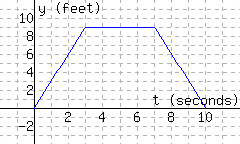
The following figure has the graph \(y=d(t)\text{,}\) which models a particle’s distance from the starting line in feet, where \(t\) stands for time in seconds since timing started.
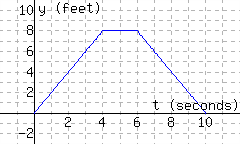
Find \(d(7)\text{.}\)
-
Interpret the meaning of \(d(7)\text{.}\)
A. In the first \(6\) seconds, the particle moved a total of \(7\) feet.
B. The particle was \(6\) feet away from the starting line \(7\) seconds since timing started.
C. The particle was \(7\) feet away from the starting line \(6\) seconds since timing started.
D. In the first \(7\) seconds, the particle moved a total of \(6\) feet.
Solve \(d(t)={4}\) for \(t\text{.}\) \(t=\)
-
Interpret the meaning of part c’s solution(s).
A. The particle was \(4\) feet from the starting line \(8\) seconds since timing started.
B. The particle was \(4\) feet from the starting line \(2\) seconds since timing started.
C. The particle was \(4\) feet from the starting line \(2\) seconds since timing started, or \(8\) seconds since timing started.
D. The particle was \(4\) feet from the starting line \(2\) seconds since timing started, and again \(8\) seconds since timing started.
100.
The following figure has the graph \(y=d(t)\text{,}\) which models a particle’s distance from the starting line in feet, where \(t\) stands for time in seconds since timing started.
Find \(d(7)\text{.}\)
-
Interpret the meaning of \(d(7)\text{.}\)
A. In the first \(9\) seconds, the particle moved a total of \(7\) feet.
B. In the first \(7\) seconds, the particle moved a total of \(9\) feet.
C. The particle was \(9\) feet away from the starting line \(7\) seconds since timing started.
D. The particle was \(7\) feet away from the starting line \(9\) seconds since timing started.
Solve \(d(t)={6}\) for \(t\text{.}\) \(t=\)
-
Interpret the meaning of part c’s solution(s).
A. The particle was \(6\) feet from the starting line \(2\) seconds since timing started, or \(8\) seconds since timing started.
B. The particle was \(6\) feet from the starting line \(8\) seconds since timing started.
C. The particle was \(6\) feet from the starting line \(2\) seconds since timing started, and again \(8\) seconds since timing started.
D. The particle was \(6\) feet from the starting line \(2\) seconds since timing started.
101.
The function \(C\) models the the number of customers in a store \(t\) hours since the store opened.
| \(t\) | \(0\) | \(1\) | \(2\) | \(3\) | \(4\) | \(5\) | \(6\) | \(7\) |
| \(C(t)\) | \(0\) | \(48\) | \(78\) | \(102\) | \(101\) | \(78\) | \(39\) | \(0\) |
Find \(C(6)\text{.}\)
-
Interpret the meaning of \(C(6)\text{.}\)
A. There were \(39\) customers in the store \(6\) hours after the store opened.
B. In \(6\) hours since the store opened, the store had an average of \(39\) customers per hour.
C. In \(6\) hours since the store opened, there were a total of \(39\) customers.
D. There were \(6\) customers in the store \(39\) hours after the store opened.
Solve \(C(t)=78\) for \(t\text{.}\) \(t=\)
-
Interpret the meaning of Part c’s solution(s).
A. There were \(78\) customers in the store \(2\) hours after the store opened.
B. There were \(78\) customers in the store \(2\) hours after the store opened, and again \(5\) hours after the store opened.
C. There were \(78\) customers in the store \(5\) hours after the store opened.
D. There were \(78\) customers in the store either \(2\) hours after the store opened, or \(5\) hours after the store opened.
102.
Suppose that \(f\) is the function that tells you how many dimes are in \(x\) dollars. Write a formula for \(f\text{.}\)
103.
Let \(f(t)\) denote the number of people eating in a restaurant \(t\) minutes after 5 PM. Answer the following questions:
a) Which of the following statements best describes the significance of the expression \(f( 5 ) = 17\text{?}\)
There are 5 people eating at 5:17 PM
Every 5 minutes, 17 more people are eating
There are 17 people eating at 5:05 PM
There are 17 people eating at 10:00 PM
None of the above
b) Which of the following statements best describes the significance of the expression \(f(a) = 28\text{?}\)
\(a\) hours after 5 PM there are 28 people eating
Every 28 minutes, the number of people eating has increased by \(a\) people
\(a\) minutes after 5 PM there are 28 people eating
At 5:28 PM there are \(a\) people eating
None of the above
c) Which of the following statements best describes the significance of the expression \(f( 28 ) = b\text{?}\)
\(b\) hours after 5 PM there are 28 people eating
At 5:28 PM there are \(b\) people eating
Every 28 minutes, the number of people eating has increased by \(b\) people
\(b\) minutes after 5 PM there are 28 people eating
None of the above
d) Which of the following statements best describes the significance of the expression \(n=f(t)\text{?}\)
\(t\) hours after 5 PM there are \(n\) people eating
\(n\) minutes after 5 PM there are \(t\) people eating
Every \(t\) minutes, \(n\) more people have begun eating
\(n\) hours after 5 PM there are \(t\) people eating
None of the above
104.
Let \(s(t)={10t^{2}-2t+100}\text{,}\) where \(s\) is the position (in mi) of a car driving on a straight road at time \(t\) (in hr). The car’s velocity (in mi/hr) at time \(t\) is given by \(v(t)={20t-2}\text{.}\)
Using function notation, express the car’s position after \(1.8\) hours. The answer here is not a formula, it’s just something using function notation like
f(8).Where is the car then? The answer here is a number with units.
Use function notation to express the question, “When is the car going \({64\ {\textstyle\frac{\rm\mathstrut mi}{\rm\mathstrut hr}}}\text{?}\)” The answer is an equation that uses function notation; something like
f(x)=23. You are not being asked to actually solve the equation, just to write down the equation.Where is the car when it is going \({58\ {\textstyle\frac{\rm\mathstrut mi}{\rm\mathstrut hr}}}\text{?}\) The answer here is a number with units. You are being asked a question about its position, but have been given information about its speed.
105.
Let \(s(t)={10t^{2}+3t+200}\text{,}\) where \(s\) is the position (in mi) of a car driving on a straight road at time \(t\) (in hr). The car’s velocity (in mi/hr) at time \(t\) is given by \(v(t)={20t+3}\text{.}\)
Using function notation, express the car’s position after \(3.7\) hours. The answer here is not a formula, it’s just something using function notation like
f(8).Where is the car then? The answer here is a number with units.
Use function notation to express the question, “When is the car going \({63\ {\textstyle\frac{\rm\mathstrut mi}{\rm\mathstrut hr}}}\text{?}\)” The answer is an equation that uses function notation; something like
f(x)=23. You are not being asked to actually solve the equation, just to write down the equation.Where is the car when it is going \({23\ {\textstyle\frac{\rm\mathstrut mi}{\rm\mathstrut hr}}}\text{?}\) The answer here is a number with units. You are being asked a question about its position, but have been given information about its speed.
106.
Describe your own example of a function that has real context to it. You will need some kind of input variable, like “number of years since 2000” or “weight of the passengers in my car.” You will need a process for using that number to bring about a different kind of number. The process does not need to involve a formula; a verbal description would be great, as would a formula.
Give your function a name. Write the symbol(s) that you would use to represent input. Write the symbol(s) that you would use to represent output.
107.
Use the given graph of a function \(f\text{,}\) along with \(a, b, c, d, e\text{,}\) and \(h\) to answer the following questions. Some answers are points, and should be entered as ordered pairs. Some answers ask you to solve for \(x\text{,}\) so the answer should be in the form x=...
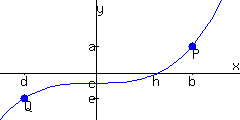
What are the coordinates of the point \(P\text{?}\)
What are the coordinates of the point \(Q\text{?}\)
Evaluate \(f(b)\text{.}\) (The answer is symbolic, not a specific number.)
Solve \(f(x)=e\) for \(x\text{.}\) (The answer is symbolic, not a specific number.)
Suppose \(c=f(z)\text{.}\) Solve the equation \(z=f(x)\) for \(x\text{.}\)